

Microcontroller based applied digital control (D. Ibrahim, 2006)
.pdf
|
FURTHER READING |
185 |
[Evans, 1954] |
Evans, W.R. Control System Dynamics, McGraw-Hill, New York, 1954. |
|
[Houpis and Lamont, 1962] |
Houpis, C.H. and Lamont, G.B. Digital Control Systems: Theory, Hardware, Soft- |
|
|
ware, 2nd edn., McGraw-Hill, New York, 1962. |
|
[Hsu and Meyer, 1968] |
Hsu, J.C. and Meyer, A.U. Modern Control Principles and Applications. McGraw- |
|
|
Hill, New York, 1968. |
|
[Jury, 1958] |
Jury, E.I. Sampled-Data Control Systems. John Wiley & Sons, Inc., New York, 1958. |
|
[Katz, 1981] |
Katz, P. Digital Control Using Microprocessors. Prentice Hall, Englewood Cliffs, NJ, |
|
|
1981. |
|
[Kuo, 1963] |
Kuo, B.C. Analysis and Synthesis of Sampled-Data Control Systems. Prentice Hall, |
|
|
Englewood Cliffs, NJ, 1963. |
|
[Lindorff, 1965] |
Lindorff, D.P. Theory of Sampled-Data Control Systems. John Wiley & Sons, Inc., |
|
|
New York, 1965. |
|
[Ogata, 1990] |
Ogata, K. Modern Control Engineering, 2nd edn., Prentice Hall, Englewood Cliffs, |
|
|
NJ, 1990. |
|
[Phillips and Harbor, 1988] |
Phillips, C.L. and Harbor R.D. Feedback Control Systems. Englewood Cliffs, NJ, |
|
|
Prentice Hall, 1988. |
|
[Raven, 1995] |
Raven, F.H. Automatic Control Engineering, 5th edn., McGraw-Hill, New York, 1995. |
|
[Strum and Kirk, 1988] |
Strum, R.D. and Kirk D.E. First Principles of Discrete Systems and Digital Signal |
|
|
Processing. Addison-Wesley, Reading, MA, 1988. |
|

8
System Stability
This chapter is concerned with the various techniques available for the analysis of the stability of discrete-time systems.
Suppose we have a closed-loop system transfer function
Y (z) |
= |
|
G(z) |
= |
N (z) |
||||
|
|
|
|
|
|
|
, |
||
R(z) |
1 |
+ |
GH(z) |
D(z) |
|||||
|
|
|
|
|
|
|
|
|
|
where 1 + GH(z) = 0 is also known as the characteristic equation. The stability of the system depends on the location of the poles of the closed-loop transfer function, or the roots of the characteristic equation D(z) = 0. It was shown in Chapter 7 that the left-hand side of the s-plane, where a continuous system is stable, maps into the interior of the unit circle in the z- plane. Thus, we can say that a system in the z-plane will be stable if all the roots of the characteristic equation, D(z) = 0, lie inside the unit circle.
There are several methods available to check for the stability of a discrete-time system:
Factorize D(z) = 0 and find the positions of its roots, and hence the position of the closedloop poles.
Determine the system stability without finding the poles of the closed-loop system, such as Jury’s test.
Transform the problem into the s-plane and analyse the system stability using the wellestablished s-plane techniques, such as frequency response analysis or the Routh–Hurwitz criterion.
Use the root-locus graphical technique in the z-plane to determine the positions of the system poles.
The various techniques described in this section will be illustrated with examples.
8.1 FACTORIZING THE CHARACTERISTIC EQUATION
The stability of a system can be determined if the characteristic equation can be factorized. This method has the disadvantage that it is not usually easy to factorize the characteristic equation. Also, this type of test can only tell us whether or not a system is stable as it is. It does not tell us about the margin of stability or how the stability is affected if the gain or some other parameter is changed in the system.
Microcontroller Based Applied Digital Control D. Ibrahim
C 2006 John Wiley & Sons, Ltd. ISBN: 0-470-86335-8
188 System Stability
|
|
|
|
e(s) |
e*(s) |
1 − e−Ts |
|
|
|
|
|
|
|
y(s) |
|||
r(s) |
|
|
|
4 |
|
|
|
||||||||||
|
|
|
|
|
|
|
s |
|
|
|
|
|
|
|
|
|
|
|
− |
|
|
|
|
|
|
s + |
2 |
|
|
|
|||||
+ |
|
|
|
|
|
|
|
|
|
|
|||||||
|
|
|
|
|
|
|
|
|
|
||||||||
|
|
|
|
|
|
|
|
|
|
|
|
|
|
||||
|
|
|
|
|
|
|
|
|
|
|
|
|
|
|
|
|
|
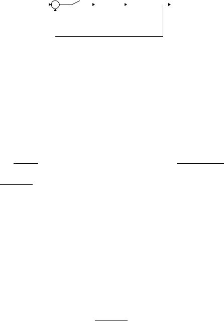
Figure 8.1 Closed-loop system
Example 8.1
The block diagram of a closed-loop system is shown in Figure 8.1. Determine whether or not the system is stable. Assume that T = 1 s.
Solution
The closed-loop system transfer function is
Y (z) |
= |
|
G(z) |
(8.1) |
||
|
|
|
|
, |
||
R(z) |
1 |
+ |
G(z) |
|||
|
|
|
|
|
|
|
where
1 − e−T s
G(z) = Z
s
= 2(1 − e−2T ) . z − e−2T
For T = 1 s,
|
4 |
|
|
|
(1 |
|
z−1)Z |
|
|
|
4 |
|
|
|
|
(1 |
|
z−1) |
|
2z(1 − e−2T ) |
|
||||||
s |
|
2 |
|
= |
− |
s(s |
|
|
2) |
|
= |
− |
|
|
|||||||||||||
+ |
|
|
|
+ |
|
(z |
− |
1)(z |
− |
e |
− |
2T ) |
|||||||||||||||
|
|
|
|
|
|
|
|
|
|
|
|
|
|
|
|
|
|
|
|
|
|
||||||
|
|
|
|
|
|
|
|
|
|
|
|
|
|
|
|
|
|
|
|
|
|
|
|
|
(8.2) |
||
|
|
|
|
|
G(z) = |
|
1.729 |
|
. |
|
|
|
|
|
|
|
|
|
|
|
|
|
|
||||
|
|
|
|
|
|
|
|
|
|
|
|
|
|
|
|
|
|
|
|
|
|
||||||
|
|
|
|
|
z |
− |
0.135 |
|
|
|
|
|
|
|
|
|
|
|
|
|
|
||||||
|
|
|
|
|
|
|
|
|
|
|
|
|
|
|
|
|
|
|
|
|
|
|
|
|
|
|
|
The roots of the characteristic equation are 1 + G(z) = 0, or 1 + 1.729/(z − 0.135) = 0, the solution of which is z = −1.594 which is outside the unit circle, i.e. the system is not stable.
Example 8.2
For the system given in Example 8.1, find the value of T for which the system is stable.
Solution
From (8.2),
G(z) = 2(1 − e−2T ) . z − e−2T
The roots of the characteristic equation are 1 + G(z) = 0, or 1 + 2(1 − e−2T )/(z − e−2T ) = 0, giving
z − e−2T + 2(1 − e−2T ) = 0

JURY’S STABILITY TEST |
189 |
or
z = 3e−2T − 2.
The system will be stable if the absolute value of the root is inside the unit circle, i.e.
|3e−2T − 2|< 1,
from which we get
2T < ln |
31 |
or T < 0.549. |
Thus, the system will be stable as long as the sampling time T < 0.549.
8.2 JURY’S STABILITY TEST
Jury’s stability test is similar to the Routh–Hurwitz stability criterion used for continuoustime systems. Although Jury’s test can be applied to characteristic equations of any order, its complexity increases for high-order systems.
To describe Jury’s test, express the characteristic equation of a discrete-time system of order n as
F (z) = an zn + an−1zn−1 + . . . + a1z + a0 = 0, |
(8.3) |
where an > 0. We now form the array shown in Table 8.1. The elements of this array are defined as follows:
The elements of each of the even-numbered rows are the elements of the preceding row, in reverse order.
The elements of the odd-numbered rows are defined as:
bk |
|
an |
ak |
, |
ck |
|
nn 1 |
bk |
, |
dk |
|
cn 2 |
ck |
, |
|
. |
|||
|
= |
|
a0 |
an−k |
|
|
= |
|
b0 |
bn−k−1 |
|
|
= |
|
c0 |
cn−2−k |
|
· · · |
|
|
|
|
|
− |
|
|
− |
|
|
||||||||||
|
|
|
|
|
|
|
|
|
|
|
|
|
|
|
|
|
|
|
|
|
|
|
|
|
|
|
|
|
|
|
|
|
|
|
|
|
|
|
|
Table 8.1 Array for Jury’s stability tests
z0 |
z1 |
z2 |
. . . |
zn−k |
. . . |
zn−1 |
zn |
a0 |
a1 |
a2 |
. . . |
an−k |
. . . |
an−1 |
an |
an |
an−1 |
an−2 |
. . . |
ak |
. . . |
a1 |
a0 |
b0 |
b1 |
b2 |
. . . |
bn−k |
. . . |
bn−1 |
|
bn−1 |
bn−2 |
bn−3 |
. . . |
bk−1 |
. . . |
b0 |
|
c0 |
c1 |
c2 |
. . . |
cn−k |
. . . |
|
|
cn−2 |
cn−3 |
cn−4 |
. . . |
ck−2 |
. . . |
|
|
. . . |
. . . |
. . . |
. . . |
. . . |
|
|
|
. . . |
. . . |
. . . |
. . . |
. . . |
|
|
|
l0 |
l1 |
l2 |
l3 |
|
|
|
|
l3 |
l2 |
l1 |
l0 |
|
|
|
|
m0 |
m1 |
m2 |
|
|
|
|
|
190 System Stability
The necessary and sufficient conditions for the characteristic equation (8.3) to have roots inside the unit circle are given as
F (1) > 0, (−1)n F (−1) > 0, |a0|< an ,
|b0| > bn−1 |c0| > cn−2 |d0| > dn−3
. . .
. . .
|m0| > m2.
Jury’s test is then applied as follows:
(8.4)
(8.5)
Check the three conditions given in (8.4) and stop if any of these conditions is not satisfied.
Construct the array given in Table 8.1 and check the conditions given in (8.5). Stop if any condition is not satisfied.
Jury’s test can become complex as the order of the system increases. For systems of order 2 and 3 the test reduces to the following simple rules. Given the second-order system characteristic equation
F (z) = a2z2 + a1z + a0 = 0, where a2 > 0,
no roots of the system characteristic equation will be on or outside the unit circle provided that
F (1) > 0, F (−1) > 0, |a0|< a2..
Given the third-order system characteristic equation
F (z) = a3z3 + a2z2 + a1z + a0 = 0, where a3 > 0,
no roots of the system characteristic equation will be on or outside the unit circle provided that
F (1) > 0, |
F (−1) < 0, |
|a0|< a3, |
||||||
det |
a3 |
a0 |
|
> |
det |
a3 |
a2 |
. |
|
a0 |
a3 |
|
|
|
a0 |
a1 |
|
|
|
|
|
|
|
|
|
|
|
|
|
|
|
|
|
|
|
Examples are given below.
Example 8.3
The closed-loop transfer function of a system is given by
|
|
|
G(z) |
|||
|
|
|
|
|
, |
|
|
|
|
|
|
||
where |
|
1 + G(z) |
||||
|
|
|
|
|
|
|
G(z) |
|
|
|
0.2z + 0.5 |
. |
|
= z2 |
|
|||||
|
− 1.2z + 0.2 |
|||||
Determine the stability of this system using Jury’s test.

|
|
|
|
|
|
|
JURY’S STABILITY TEST |
191 |
|||
Solution |
|
|
|
|
|
|
|
|
|
|
|
The characteristic equation is |
|
|
|
|
|
|
|
|
|
|
|
1 |
|
|
G(z) |
|
1 |
|
0.2z + 0.5 |
|
0 |
|
|
|
+ |
= |
+ z2 − 1.2z + 0.2 |
= |
|
||||||
or |
|
|
|
|
|
||||||
|
|
|
|
|
|
|
|
|
|
|
|
|
|
|
|
z2 − z + 0.7 = 0. |
|
|
|
||||
Applying Jury’s test, |
|
|
|
|
|
|
|
|
|
|
|
F (1) = 0.7 > 0, |
|
F (−1) = 2.7 > 0, |
0.7 < 1. |
|
|||||||
All the conditions are satisfied and the system is stable. |
|
|
|
||||||||
Example 8.4 |
|
|
|
|
|
|
|
|
|
|
|
The characteristic equation of a system is given by |
|
|
|
||||||||
1 |
|
|
G(z) |
|
1 |
|
K (0.2z + 0.5) |
|
|
0. |
|
+ |
= |
+ z2 − 1.2z + 0.2 |
= |
|
|||||||
|
|
|
|
|
|||||||
Determine the value of K for which the system is stable. |
|
|
|
||||||||
Solution |
|
|
|
|
|
|
|
|
|
|
|
The characteristic equation is |
|
|
|
|
|
|
|
|
|
|
|
z2 + z(0.2K − 1.2) + 0.5K = 0, where K > 0. |
|
||||||||||
Applying Jurys’s test, |
|
|
|
|
|
|
|
|
|
|
|
F (1) = 0.7K − 0.2 > 0, |
F (−1) = 0.3K + 2.2 > 0, 0.5K < 1. |
|
|||||||||
Thus, the system is stable for 0.285 < K < 2.
Example 8.5
The characteristic equation of a system is given by
F (z) = z3 − 2z2 + 1.4z − 0.1 = 0.
Determine the stability of the system.
Solution |
|
|
|
|
|
|
|
|
|
|
|
|
|
|
|
|
|
||
Applying Jury’s test, a3 = 1, a2 = −2, a1 = 1.4, a0 = −0.1 and |
|
|
|
||||||||||||||||
|
|
|
|
|
|
F (1) = 0.3 > 0, F (−1) = −4.5 < 0, |
0.1 < 1. |
|
|||||||||||
The first conditions are satisfied. Applying the other condition, |
|
|
|
|
|||||||||||||||
|
|
|
|
|
−1 |
|
|
0.1 |
|
|
0.99 and |
−1 |
|
2 |
|
1.2; |
|||
|
|
|
|
|
|
0.1 |
1 |
|
= − |
|
|
0.1 |
1.4 |
|
= − |
|
|||
|
|
|
|
|
|
|
− |
|
|
|
− |
|
|
||||||
|
|
|
|
|
|
|
|
|
|
|
|
|
|
|
|
|
|
||
since |
| |
0.99 |
| |
< |
|
1.2 |
| |
, the |
|
|
|
|
|
|
|
|
|
|
|
|
|
|
| − |
|
|
system is not stable. |
|
|
|
|
|
|
|
||||||
|
|
|
|
|
|
|
|
|
|
|
|
|
|
|
|
||||

192 System Stability
8.3 ROUTH–HURWITZ CRITERION
The stability of a sampled data system can be analysed by transforming the system characteristic equation into the s-plane and then applying the well-known Routh–Hurwitz criterion.
A bilinear transformation is usually used to transform the left-hand s-plane into the interior of the unit circle in the z-plane. For this transformation, z is replaced by
|
= |
1 |
|
w |
|
|
z |
|
1 |
+ w |
. |
(8.6) |
|
|
|
|||||
|
|
|
− |
|
|
|
Given the characteristic equation in w,
F (w) = bn wn + bn−1wn−1 + . . . + b1w + b0 = 0,
then the Routh–Hurwitz array is formed as follows:
wn−1 |
bn n |
1 |
bn−3 |
bn−5 . . . |
|
wn |
|
b |
|
bn 2 |
bn 4 . . . |
wn−2 |
− |
|
− |
− |
|
|
c1 |
|
c2 |
c3 . . . |
|
|
|
|
|
|
|
. . . |
. . . . . . . . . . . . |
||||
|
|
|
|
|
|
w1 |
|
j1 |
|
|
|
|
|
|
|
|
|
w0 |
|
k1 |
|
|
|
The first two rows are obtained from the equation directly and the other rows are calculated as follows:
c1 = bn−1bn−2 − bn bn−3 ,
bn−1
c2 = bn−1bn−4 − bn bn−5 , bn−1
c3 = bn−1bn−6 − bn bn−7 ,
bn−1
d1 = c1bn−3 − bn−1c2 , c1
. . . .
The Routh–Hurwitz criterion states that the number of roots of the characteristic equation in the right hand s-plane is equal to the number of sign changes of the coefficients in the first column of the array. Thus, for a stable system all coefficients in the first column must have the same sign.
Example 8.6
The characteristic equation of a sampled data system is given by
z2 − z + 0.7 = 0.
Determine the stability of the system using the Routh–Hurwitz criterion.
Solution
Transforming the characteristic equation into the w-plane gives
1 |
+ w |
2 |
− 1 |
+ w + 0.7 = 0, |
|||
|
1 |
w |
|
|
1 |
w |
|
|
|
− |
|
|
|
− |
|
|
|
|
|
|
ROUTH–HURWITZ CRITERION |
193 |
||||||
|
|
|
|
|
|
|
|
|
|
|
|
|
r(s) |
e(s) |
e*(s) |
1 − e−Ts |
|
|
|
K |
|
y(s) |
|
||
+ |
− |
|
|
s |
|
|
|
s(s + 1) |
|
|
|
|
|
|
|
|
|
|
|
|
|
|
|
||
|
|
|
|
|
|
|
|
|
|
|
|
|
|
|
|
|
|
|
|
|
|
|
|
|
|
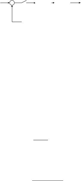
Figure 8.2 Closed-loop system
or
2.7w2 + 0.6w + 0.7 = 0.
Forming the Routh–Hurwitz array,
w2 2.7 0.7
w1 0.6 0 w0 0.7
there are no sign changes in the first column and thus the system is stable.
Example 8.7
The block diagram of a sampled data system is shown in Figure 8.2. Use the Routh–Hurwitz criterion to determine the value of K for which the system is stable. Assume that K > 0 and T = 1 s.
Solution |
|
|
|
|
|
|
|
|
|
|
|
|
|
|
|
|
|
|
|
|
|
|
The characteristic equation is 1 + G(z) = 0, where |
|
|
|
|
|
|
|
|
|
|||||||||||||
|
G(s) |
= |
|
1 − e−T s |
|
|
|
|
K |
. |
|
|
||||||||||
|
|
|
|
|
|
|
|
|
|
|||||||||||||
|
|
|
|
|
|
s |
|
|
s(s |
+ |
1) |
|
|
|
|
|||||||
|
|
|
|
|
|
|
|
|
|
|
|
|
|
|||||||||
The z-transform is given by |
|
|
|
|
|
|
|
|
|
|
|
|
|
|
|
|
|
|
|
|
|
|
G(z) = (1 − z−1)Z |
K |
|
|
|
|
, |
||||||||||||||||
s2(s |
|
1) |
||||||||||||||||||||
which gives |
|
|
|
|
|
|
|
|
|
|
|
|
|
|
+ |
|
|
|
|
|
||
|
|
|
|
|
|
|
|
|
|
|
|
|
|
|
|
|
|
|
|
|
|
|
G(z) |
= |
K (0.368z + 0.264) |
. |
|
||||||||||||||||||
|
|
|
(z |
− |
1)(z |
− |
0.368) |
|
|
|
||||||||||||
|
|
|
|
|
|
|
|
|
|
|||||||||||||
The characteristic equation is |
|
|
|
|
|
|
|
|
|
|
|
|
|
|
|
|
|
|
|
|
|
|
1 |
+ |
K (0.368z + 0.264) |
|
= |
0, |
|
||||||||||||||||
|
|
|||||||||||||||||||||
|
(z |
− |
1)(z |
− |
0.368) |
|
|
|
|
|
||||||||||||
|
|
|
|
|
|
|
|
|
||||||||||||||
or
z2 − z(1.368 − 0.368K ) + 0.368 + 0.264K = 0.

194 System Stability
Transforming into the w-plane gives
|
1 |
w |
2 |
1 |
w |
|
|
|
||
|
|
|
|
|
||||||
|
|
|
+ |
− |
|
+ |
(1.368 − 0.368K ) + 0.368 + 0.264K = 0 |
|||
1 |
w |
1 |
w |
|||||||
or |
|
|
− |
|
|
− |
|
|
|
|
|
|
|
|
|
|
|
|
|
|
|
|
|
|
w2(2.736 − 0.104K ) + w(1.264 − 0.528K ) + 0.632K = 0. |
|||||||
We can now form the Routh–Hurwitz array |
|
|||||||||
|
|
|
|
|
|
w2 |
|
2.736 |
0.104K |
0.632K |
|
|
|
|
|
|
w1 |
1.264 − |
0.528K |
0 |
|
|
|
|
|
|
|
w0 |
|
− |
|
|
|
|
|
|
|
|
|
0.632K |
|
||
The system is stable if there is no sign change in the first column. Thus, for stability,
1.264 − 0.528K > 0
or
K < 2.4.
8.4 ROOT LOCUS
The root locus is one of the most powerful techniques used to analyse the stability of a closedloop system. This technique is also used to design controllers with required time response characteristics. The root locus is a plot of the locus of the roots of the characteristic equation as the gain of the system is varied. The rules of the root locus for discrete-time systems are identical to those for continuous systems. This is because the roots of an equation Q(z) = 0 in the z-plane are the same as the roots of Q(s) = 0 in the s-plane. Even though the rules are the same, the interpretation of the root locus is quite different in the s-plane and the z-plane. For example, a continuous system is stable if the roots are in the left-hand s-plane. A discrete-time system, on the other hand, is stable if the roots are inside the unit circle. The construction and the rules of the root locus for continuous-time systems are described in many textbooks. In this section only the important rules for the construction of the discrete-time root locus are given, with worked examples.
Given the closed-loop system transfer function
G(z)
,
1 + GH(z)
we can write the characteristic equation as 1 + k F (z) = 0, and the root locus can then be plotted as k is varied. The rules for constructing the root locus can be summarized as follows:
1.The locus starts on the poles of F (z) and terminate on the zeros of F (z).
2.The root locus is symmetrical about the real axis.
3.The root locus includes all points on the real axis to the left of an odd number of poles and zeros.
ROOT LOCUS |
195 |
4. If F (z) has zeros at infinity, the root locus will have asymptotes as k → ∞. The number of asymptotes is equal to the number of poles n p , minus the number of zeros nz . The angles of the asymptotes are given by
180r
θ = , where r = ±1, ±3, ±5, . . . .
n p − nz
The asymptotes intersect the real axis at σ , where
σ = |
poles of F (n |
− n |
zeros of F (z) . |
|
z) |
|
|
p − z
5. The breakaway points on the real axis of the root locus are at the roots of
dF(z) = 0.
dz
6.If a point is on the root locus, the value of k is given by
1 + kF(z) = 0 or k = − 1 .
F (z)
Example 8.8
A closed-loop system has the characteristic equation
1 + GH(z) = 1 + K 0.368(z + 0.717) = 0. (z − 1)(z − 0.368)
Draw the root locus and hence determine the stability of the system.
Solution
Applying the rules:
1. The above equation is in the form 1 + kF(z) = 0, where
F (z) = 0.368(z + 0.717) . (z − 1)(z − 0.368)
The system has two poles at z = 1 and at z = 0.368. There are two zeros, one at z = −0.717 and the other at minus infinity. The locus will start at the two poles and terminate at the two zeros.
2.The section on the real axis between z = 0.368 and z = 1 is on the locus. Similarly, the section on the real axis between z = −∞ and z = −0.717 is on the locus.
3. Since n p − nz = 1, there is one asymptote and the angle of this asymptote is
θ |
|
180r |
|
180◦ |
|
for r |
|
1. |
= n p − nz |
= ± |
|
= ± |
|||||
|
|
|
180◦ |
|
||||
Note that since the angles of the asymptotes are |
± |
it is meaningless to find the real |
||||||
|
|
|
|
|
|
|
|
|
axis intersection point of the asymptotes.