Mathematics for Life Sciences and Medicine - Takeuchi Iwasa and Sato

216 H.I. Freedman

into the first equation of (20) and writing p1(x+1) = x+1p61(x+1) (since p1(0) = 0 and p1(0) exists), we get that for x+1 > 0,

Note that p61(0) = p1(0) > 0. Writing (22) as F1(x+1) = G1(x+1), we easily see that F1(0) = α1γ > 0, F1(K1) = 0, G1(0) = δp1(0), G1(K1) = δp61(K1) > 0. Since by hypothesis F1(0) > G1(0) and F1(K1) < G1(K1), there exists a 0 <

x+1 < K1 such that (22) holds. Then from (21), h(y+) > 0 exists and therefore y+ > 0 exists.

To check whether E exists, one must solve the full algebraic system, writing pi(xi) = xip6i(xi), i = 1, 2,

It is extremely di cult to see whether or not system (25) has a positive solution. Hence we take a di erent approach to obtain criteria for the existence of E , namely persistence theory. In order to do so, we will need the

−η1p1(0)h(y+2) −η2p2(x+2)h(y+2) −[γ + η2p2(x+2)]h (y+2)

First we examine M0. The eigenvalues of M0 are given by

α1 − p1(0)h(y0) , α2 − p2(0)h(y0) and − γh (y0) .

From this, E0 is clearly locally stable in the y direction and is locally stable or unstable in the xi direction according to whether αi − pi(0)h(y0) is negative or positive.

The important concern is with α2 − p2(0)h(y0), for if this expression is negative, then cancer can be eradicated if caught in time. However, at the same time we would want α1 − p1(0)h(y0) > 0 so that the healthy cells survive.

Finally for persistence to hold according to techniques developed in Freed-

man and Waltman (1984), we would require 0 to be unstable, and for +i to

E E

be unstable locally in the j direction, i, j = 1, 2, j = i. Hence the criteria for persistence are as follows:

Finally from results given in Butler et al. (1986), if (26) holds, then E exists.

9.4.2 Periodic treatment

In actual practice, a form of periodic treatment is employed. Typically, the cancer patient is given a fixed number of doses over a fixed period of time at regular intervals. This may be approximated by a periodic step function.

Here w(t) is the concentration of lymphocytes z(t) is the concentration of LAC cells, f (w, z) is the rate of lymphocyte proliferation due to the influence of LAC cells, h(x2, z) is the rate of cancer destruction by lymphocytes and Qi are the respective rates of infusion of lymphocytes and LAC cells into the body. γ1e1(w) and γ2e2(z) are the natural death or washout rates of the lymphocytes and LAC cells respectively. δ is the proportionate combination of lymphocytes with cancer cells, and η is the proportionate influence of the lymphocytes on LAC cells. It is shown in Nani and Freedman (2000) that solutions of system (28) enter into a bounded invariant region and that the system is dissipative.

There are four possible equilibria for system (28) of the form

E3(x1 , x2 , w , z ) .

The equilibrium of interest is E1, for if E1 is locally stable in the x2 direction, then cancer could be eradicated if caught early enough. The variational

Then the local stability in the x2 direction is given by g(w) = α2 − β2K1 − hx2 (0, w) assuming hw (0, w) = 0 given the definition of h(x2, w). Hence if g(w) < 0, cancer can be eradicated if caught early enough.

System (28) is analyzed in detail in Nani and Freedman (2000).

220 H.I. Freedman

9.6 Metastasis

Metastasis means that the cancer has spread from one site to another. Usually the metastasis occurs one way only. It is very often the case that the cancer at the second site is much more deadly than at the first site. The material from this section is taken from Pinho et al. (2002).

We consider cancer at two sites treated by chemotherapy. This requires a system of six ODE’s. We let x1(t) and x2(t) be the concentration of healthy and cancer cells respectively at the primary site and u1(t) and u2(t) be the concentration of healthy cells and cancer cells respectively at the secondary site. We further let y(t) and z(t) be the concentration of chemotherapy agent at the primary and secondary sites respectively. Thus our model becomes

(29) where we have chosen specific functional responses for simplicity and all other constants have similar interpretations as before.

Here the new feature in this model is the introduced delay term in the fifth equation, εθx2(t − τ ), which represents the fact that it takes time τ for the cancer growth to be triggered at the secondary site. Here θ is the proportion of cancer cells from the first site that are activated at the secondary site, ai are the respective Michaelis-Menton growth constants for xi, and bi are similar for ui. Note that system (29) simulates the continuous treatment case.

System (29) has nine possible equilibria of the form

F8(x1 , x2, y , u1, u2, z ) .

These are extremely di cult to analyze analytically. Here we will give some numerical results. A more detailed analysis can be found in Pinho et al. (2002).

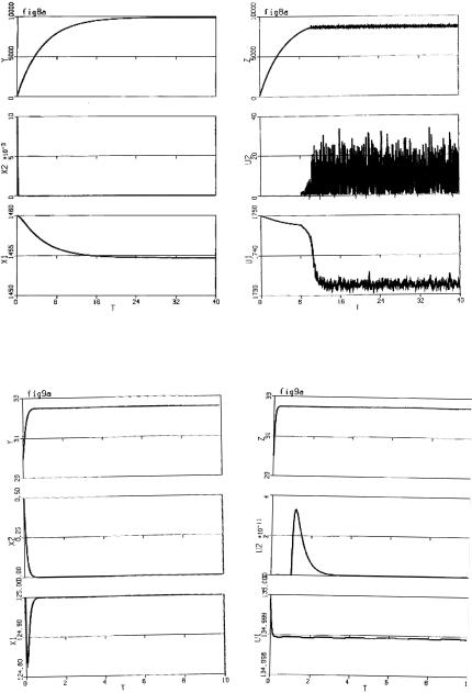
The following three figures indicate a variety of behaviours of solutions, depending on parameters and initial conditions.

In Fig. 9.3, we see that at the primary site, cancer is eradicated, but at the secondary site after time τ, the cancer takes over and drives the healthy cells to extinction. Unfortunately, this is all too often the case.

In Fig. 9.4, the behaviour at the primary site is the same as in Fig. 9.3, but at the secondary site, wild chaotic oscillations occur. This unpredictability makes it extremely di cult to prescribe treatment. This corresponds to cases where cancer seems to go in and out of remission until the body succumbs.

Finally Fig. 9.5 shows that for certain cancers and chemotherapies, the cancer can be controlled at both sites.

Fig. 9.3. a Cancer eradicated at primary site. b Cancer outcompetes normal cells at secondary site

222 H.I. Freedman

Fig. 9.4. a Cancer eradicated at primary site. b Chaotic behavior at secondary site

Fig. 9.5. Cancer eradicated at both primary and secondary sites

Index

References

1.Agur, Z., R. Arnon and B. Schector (1992), E ect of dosing interval on myelotoxicity and survival in mice treated by cytarabine, Eur. J. Cancer 28, 1085– 1090.
2.Belostotski, G. (2004), A Control Theory Model for Cancer Treatment by Radiotherapy, M.Sc. Thesis, University of Alberta.
3.Butler, G.J., H.I. Freedman and P. Waltman (1986), Uniformly persistent systems, Proc. Amer. Math. Soc. 96, 425–430.
4.Freedman, H.I. and P. Waltman (1984), Persistence in models of three interacting predator-prey populations, Math. Biosci. 68, 213–231.
5.Freedman, H.I. (1980), Deterministic Mathematical Models in Population Ecology, Marcel Dekker, New York.
6.Horn, M.A. and G. Webb (2004), Discrete and continuous dynamical systems 4, 1–348, special issue on Mathematical Models in Cancer.
7.Nani, F. and H.I. Freedman (2000), A mathematical model of cancer treatment of immunotherapy, Math. Biosci. 163, 159–199.
8.Nani, F. (1998), Mathematical Models of Chemotherapy and Immunotherapy, Ph.D. Thesis, University of Alberta.
9.Pinho, S.T.R., H.I. Freedman and F. Nani (2002), A chemotherapy model for the treatment of cancer with metastasis, Math. Comput. Model 36, 773–803.
10.Pliss, V.A. (1966), Nonlocal Problems of the Theory of Oscillations, Academic Press, New York.
11.Toledo-Pereya, L.H. (1988), Immunology Essentials for Surgical Practice, PSG, Littlestone, MA.