Mathematics for Life Sciences and Medicine - Takeuchi Iwasa and Sato

20.Lurie, M. B. (1964), Resistance to tuberculosis : experimental studies in native and acquired defensive mechanisms, Harvard Univ. Press, Cambridge, Mass.

21.Marino, S. and D. E. Kirschner (2004), The human immune response to Mycobacterium tuberculosis in lung and lymph node, J. Theor. Biol. 227 4, 463.

22. Marino, S., S. Pawar, C. L. Fuller, T. A. Reinhart, J. L. Flynn and

D.E. Kirschner, (2004), Dendritic cell tra cking and antigen presentation in the human immune response to Mycobacterium tuberculosis, J. Immunol. 173 1, 494.

23.Medzhitov R. and C. A. Janeway, Jr. (1997), Innate immunity: the virtues of a nonclonal system of recognition, Cell, 91, 295.

24.Medzhitov, R. and C. A. Janeway, Jr. (2000), Innate immunity, N. Engl.

J.Med., 343, 338.

25.Medzhitov, R. and C. A. Janeway, Jr. (2002), Decoding the patterns of self and nonself by the innate immune system. Science, 296, 298.

26.Mercer R. R., M. L. Russell, V. L. Roggli and J. D. Crapo (1994), Cell number and distribution in human and rat airways, Am. J. Respir. Cell. Mol. Biol., 10, 613.

27.Murali-Krishna, K., L. L. Lau, S. Sambhara, F. Lemonnier, J. Altman and

R.Ahmed (1999), Persistence of memory CD8 T cells in MHC class I-deficient mice, Science, 286, 1377.

28.Murray, J. D. (2002), Mathematical biology, 3rd edn., Springer, New York.

29.North R. J. and A. A. Izzo (1993), Mycobacterial virulence. Virulent strains of Mycobacteria tuberculosis have faster in vivo doubling times and are better equipped to resist growth-inhibiting functions of macrophages in the presence and absence of specific immunity, J. Exp. Med., 177, 1723.

30.Shampine, L. F. and S. Thompson, Solving DDEs with Matlab, manuscript, URL: http://www.radford.edu/ thompson/webddes

31.Silver, R. F., Q. Li, J. J. Ellner (1998b), Expression of virulence of Mycobacterium tuberculosis within human monocytes: virulence correlates with intracellular growth and induction of tumor necrosis factor alpha but not with evasion of lymphocytedependent monocyte e ector functions, Infect. Immun., 66, 1190.

32.Silver, R. F., Q. Li, W. H. Boom and J. J. Ellner (1998a), Lymphocytedependent inhibition of growth of virulent Mycobacterium tuberculosis H37Rv within human monocytes: requirement for CD4+ T cells in purified protein derivative-positive, but not in purified protein derivative-negative subjects,

J.Immunol., 160, 2408.

33.Sprent, J. and A. Basten (1973), Circulating T and B lymphocytes of the mouse.

II.Lifespan, Cell. Immunol., 7, 40.

34.Sprent, J., C. D. Surh (2002), T cell memory Annu. Rev. Immunol., 20, 551.

35.Stone, K. C., R. R. Mercer, P. Gehr, B. Stockstill and J. D. Crapo (1992), Allometric relationships of cell numbers and size in the mammalian lung, Am.

J.Respir. Cell. Mol. Biol., 6, 235.

36.Surh, C. D. and J. Sprent (2002), Regulation of naive and memory T-cell homeostasis, Microbes Infect., 4, 51.

37.Swain,S. L., H. Hu and G. Huston (1999), Class II-independent generation of CD4 memory T cells from e ectors Science, 286, 1381.

38.Takeda, K., T. Kaisho and S. Akira (2003), Toll-like receptors, Annu. Rev. Immunol., 21, 335.

206 Edoardo Beretta et al.

39.Tan, J. S., D. H. Canaday, W. H. Boom, K. N. Balaji, S. K. Schwander and E. A. Rich (1997), Human alveolar T lymphocyte responses to Mycobacterium tuberculosis antigens: role for CD4+ and CD8+ cytotoxic T cells and relative resistance of alveolar macrophages to lysis, J. Immunol., 159, 290.

40.Tsukaguchi, K., K. N. Balaji and W. H. Boom (1995), CD4+ alpha beta T cell and gamma delta T cell responses to Mycobacterium tuberculosis. Similarities and di erences in Ag recognition, cytotoxic e ector function, and cytokine production, J. Immunol., 154, 1786.

41.Van Furth, R., M. C. Diesselho -den Dulk and H. Mattie (1973), Quantitative study on the production and kinetics of mononuclear phagocytes during an acute inflammatory reaction, J. Exp. Med., 138, 1314.

42.Wigginton, J. E. and D. E. Kirschner (2001), A model to predict cell-mediated immune regulatory mechanisms during human infection with Mycobacterium tuberculosis, J. Immunol., 166, 1951.

43.Wong, P. and E. G. Pamer (2003), CD8 T cell responses to infectious pathogens,

Annu. Rev. Immunol., 21, 29.

44.Zinkernagel, R. M. (2003), On natural and artificial vaccinations, Annu. Rev. Immunol., 21, 515

9

Modeling Cancer Treatment Using

Competition: A Survey

H.I. Freedman

Summary. Several models are proposed to simulate the treatment of cancer by various techniques including chemotherapy, immunotherapy and radiotherapy. The interactions between cancer and normal cells are viewed as competitions for resources. Using ordinary di erential equations, we model these treatments as constant and periodic.

9.1 Introduction

In North America, cancer is the second largest cause of human mortality, and as such, is of great concern to the population at large. Despite the billions of dollars poured into research to date, a “cure for cancer” is still out of reach, although significant progress has been made in many types of cancers. Such progress has led to greater understanding of the cancers and their e ects and in improvements in treatments leading to a better quality of life and in some cases to a cure.

Mathematics has contributed in a small way to the understanding of cancer by analysis and simulation of cancer models in a hope of discovering new insights. This is well evidenced by the publication of a special issue of the journal, Discrete and Continuous Dynamical Systems Series B (Horn and Webb 2004), titled “Mathematical Models in Cancer”, which contains twentyone papers concerned with modelling various types and aspects of cancer. It is interesting to note, however, that in all these works (and others) there is hardly any modelling or mention of treatment.

It is the purpose of this chapter to briefly survey how treatment may be included in cancer modelling. However, we restrict ourselves to models which treat the interactions between cancer and normal cells as a competition for bodily resources (nutrients, oxygen, space, etc.).

Research partially supported by the Natural Sciences and Engineering Research Council of Canada, Grant No. NSERC OGP 4823.

include a harvesting of cells due to radiation. The general form of the new system is then given by

where ηi, i = 1, 2, is the e ect of radiation on the cell populations.

In the first instance we suppose that the radiation is ideal, i. e. it targets only cancer cells. This may be e ected by setting η1(t, x1, x2) = 0. In the second instance we can look at the case of a minor spillover to normal cells, by writing η1(t, x1, x2) = εη1(t, x1, x2), and use perturbation theory. Then at the third stage of analysis, one can consider fully system (3).

In this paper, we only consider the case where η1(t, x1, x2) = 0. For the perturbation case, see Belostotski (2004). Four types of control are feasible:

Here we will analyze in some detail case (i). The other cases may be found in Belostotski (2004).

Let

a = α1α2 − β1β2K1K2 .

In the absence of radiation, i. e. γ = 0, system (4) generates the following

The sign of a describes the nature of the interaction between healthy and

210 H.I. Freedman

cancer cells. Consider the slopes of Γ1 and Γ2 in (5). If

When a =,0the isoclines (5) do not intersect since we restrict our analysis to the case when cancer wins the competition (conditions (2)). When radiation is introduced, the equations of isoclines (5) will change to:

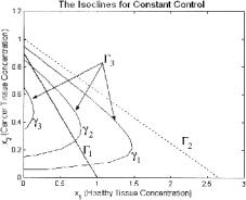
In the positive x1, x2 plane these isoclines may intersect twice, once, or zero times as in Figs. 9.1 and 9.2. The number of intersections depends on the size of γ and the dynamics of the cancer-healthy tissue interaction represented by a.

Fig. 9.1. Isoclines of (6): a < 0. Changes in shape of Γ3 for di erent values of γ : γ1 < γ2 < γ3

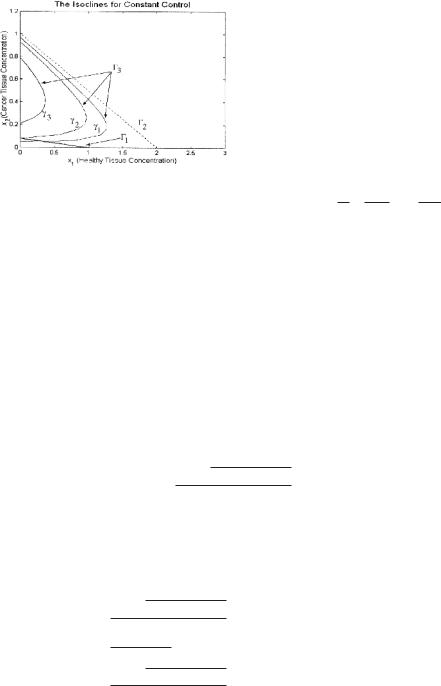
Fig. 9.2. Isoclines of (6): a < 0. Changes in shape of Γ3 for di erent values of γ : γ1 < γ2 < γ3 < γ4 < γ5

The boundary equilibria on the x2 axis will exist if 0 = αβ22 − β2αK2 2 x2 − β2γx2 or, equivalently, 0 = α2x22 − K2α2x2 + γK2 has positive solutions. Therefore,

(8) To develop conditions necessary for an internal equilibrium first we solve system (7) by substituting for x1 from the first equation into the second to obtain

where a = α1α2 − β1β2K1K2 and b = K2α1(α2 − K1β2). The solutions of this quadratic equation are given by

This x2 defines the location of an internal equilibrium. The equilibrium from now on is labeled as E = (x1, x2 ).

Conditions (2) = b > 0 since β2K1 < α2. Variable a, however, may be positive, negative, or zero. Therefore, by conditions (6), the solution to (9) are:

(

b − b2 − 4aα1K2γ

2a

is the only potential solution ,

γ

α2 −(β2K1

is the only possible solution ,

b ± b2 − 4aα1K2γ

2a

gives two potential solutions .

(11)

212 H.I. Freedman

M= ∂x1 ∂x2

∂x˙ 2 ∂x˙ 2

We would like to study the stability of the internal equilibrium, E = (x1 , x2 ). This equilibrium is found at the intersection of isoclines Γ1 and Γ3. Notice