


Data Summary and Descriptive Statistics 17
Probability Mass Function
1/6
Relative Frequency
0
1 |
2 |
3 |
4 |
5 |
6 |
Result of Toss of Single Dice
FIGURE 3.7: The probability density function for a discrete random variable (probability mass function). In this case, the random variable is the value of a toss of a single dice. Note that each of the six possible outcomes has a probability of occurrence of 1 of 6. This probability density function is also known as a uniform probability distribution.
the true probability mass function for the ideal six-sided dice. Figure 3.8 illustrates the histograms for the outcomes of 50 and 1000 tosses of a single dice. Note that even with 50 tosses or samples, it is difficult to determine what the true probability distribution might look like. However, as we approach 1000 samples, the histogram is approaching the true probability mass function (the uniform distribution) for the toss of a dice. But, there is still some variability from bin to bin that does not look as uniform as the ideal probability distribution illustrated in Figure 3.7. The message to take away from this illustration is that most biomedical research reports the outcomes of a small number of samples. It is clear from the dice example that the statistics of the underlying random process are very difficult to discern from a small sample, yet most biomedical research relies on data from small samples.
3.5GENERAL APPROACH TO STATISTICAL ANALYSIS
We have now collected our data and looked at some graphical summaries of the data. Now we will use numerical summary, also known as statistics, to try to describe the nature of the underlying population or process from which we have taken our samples. From these descriptive statistics, we assume a probability model or probability distribution for the underlying population or process and then select the appropriate statistical tests to test hypotheses or make decisions. It is important to note that the conclusions one may draw from a statistical test depends on how well the assumed probability model fits the underlying population or process.

18 introduction to statistics for bioMEDical engineers
Relative Frequency
Histogram of 50 Dice Tosses
0.2
0.1
0.0
1 |
2 |
3 |
4 |
5 |
6 |
Value of Dice Toss
Histogram of 2000 Dice Tosses
0.2
Relative Frequency
0.1
0.0
1 |
2 |
3 |
4 |
5 |
6 |
Value of Dice Toss
FIGURE 3.8: Histograms representing the outcomes of experiments in which a single dice is tossed 50 (top) and 2000 times (lower), respectively. Note that as the sample size increases, the histogram approaches the true probability distribution illustrated in Figure 3.7.
As stated in the Introduction, biomedical engineers are trying to make decisions about populations or processes to which they have limited access. Thus, they design experiments and collect samples that they think will fairly represent the underlying population or process. Regardless of what type of statistical analysis will result from the investigation or study, all statistical analysis should follow the same general approach:
Data Summary and Descriptive Statistics 19
1.Measure a limited number of representative samples from a larger population.
2.Estimate the true statistics of larger population from the sample statistics.
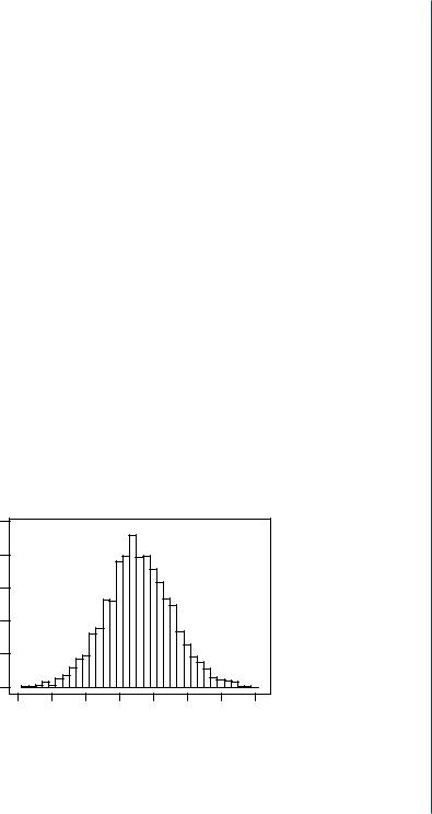
Some important concepts need to be addressed here. The first concept is somewhat obvious. It is often impossible or impractical to take measurements or observations from an entire population. Thus, the biomedical engineer will typically select a smaller, more practical sample that represents the underlying population and the extent of variability in the larger population. For example, we cannot possibly measure the resting body temperature of every person on earth to get an estimate of normal body temperature and normal range. We are interested in knowing what the normal body temperature is, on average, of a healthy human being and the normal range of resting temperatures as well as the likelihood or probability of measuring a specific body temperature under healthy, resting conditions. In trying to determine the characteristics or underlying probability model for body temperature for healthy, resting individuals, the researcher will select, at random, a sample of healthy, resting individuals and measure their individual resting body temperatures with a thermometer. The researchers will have to consider the composition and size of the sample population to adequately represent the variability in the overall population. The researcher will have to define what characterizes a normal, healthy individual, such as age, size, race, sex, and other traits. If a researcher were to collect body temperature data from such a sample of 3000 individuals, he or she may plot a histogram of temperatures measured from the 3000 subjects and end up with the following histogram (Figure 3.9).The researcher may also calculate some basic descriptive statistics for the 3000 samples, such as sample average (mean), median, and standard deviation.
Body Temperature
Density
0.5
0.4
0.3
0.2
0.1
0.0
95 |
96 |
97 |
98 |
99 |
100 |
101 |
102 |
Temperature (F)
FIGURE 3.9: Histogram for 2000 internal body temperatures collected from a normally distributed population.

20 introduction to statistics for bioMEDical engineers
Once the researcher has estimated the sample statistics from the sample population, he or she will try to draw conclusions about the larger (true) population. The most important question to ask when reviewing the statistics and conclusions drawn from the sample population is how well the sample population represents the larger, underlying population.
Once the data have been collected, we use some basic descriptive statistics to summarize the data. These basic descriptive statistics include the following general measures: central tendency, variability, and correlation.
3.6DESCRIPTIVE STATISTICS
There are a number of descriptive statistics that help us to picture the distribution of the underlying population. In other words, our ultimate goal is to assume an underlying probability model for the population and then select the statistical analyses that are appropriate for that probability model.
When we try to draw conclusions about the larger underlying population or process from our smaller sample of data, we assume that the underlying model for any sample, “event,” or measure (the outcome of the experiment) is as follows:
X = ± individual differences ± situational factors ± unknown variables,
where X is our measure or sample value and is influenced by , which is the true population mean; individual differences such as genetics, training, motivation, and physical condition; situation factors, such as environmental factors; and unknown variables such as unidentified/nonquantified factors that behave in an unpredictable fashion from moment to moment.
In other words, when we make a measurement or observation, the measured value represents or is influenced by not only the statistics of the underlying population, such as the population mean, but factors such as biological variability from individual to individual, environmental factors (time, temperature, humidity, lighting, drugs, etc.), and random factors that cannot be predicted exactly from moment to moment. All of these factors will give rise to a histogram for the sample data, which may or may not reflect the true probability density function of the underlying population. If we have done a good job with our experimental design and collected a sufficient number of samples, the histogram and descriptive statistics for the sample population should closely reflect the true probability density function and descriptive statistics for the true or underlying population. If this is the case, then we can make conclusions about the larger population from the smaller sample population. If the sample population does not reflect variability of the true population, then the conclusions we draw from statistical analysis of the sample data may be of little value.