


vii
Contents
1. |
Introduction |
....................................................................................................... |
|
1 |
|
2. |
Collecting Data and Experimental Design ............................................................ |
5 |
|||
3. |
Data Summary and Descriptive Statistics ............................................................. |
9 |
|||
|
3.1 |
Why Do We Collect Data? ................................................................................. |
9 |
||
|
3.2 |
Why Do We Need Statistics? .............................................................................. |
9 |
||
|
3.3 |
What Questions Do We Hope to Address With Our Statistical Analysis? ...... |
10 |
||
|
3.4 |
How Do We Graphically Summarize Data? ..................................................... |
11 |
||
|
|
3.4.1 |
Scatterplots ............................................................................................ |
11 |
|
|
|
3.4.2 |
Time Series ........................................................................................... |
11 |
|
|
|
3.4.3 |
Box-and-Whisker Plots ........................................................................ |
12 |
|
|
|
3.4.4 |
Histogram ............................................................................................. |
13 |
|
|
3.5 |
General Approach to Statistical Analysis .......................................................... |
17 |
||
|
3.6 |
Descriptive Statistics ......................................................................................... |
20 |
||
|
|
3.6.1 |
Measures of Central Tendency .............................................................. |
21 |
|
|
|
3.6.2 |
Measures of Variability .......................................................................... |
22 |
|
4. |
Assuming a Probability Model From the Sample Data ......................................... |
25 |
|||
|
4.1 |
The Standard Normal Distribution .................................................................. |
29 |
||
|
4.2 |
The Normal Distribution and Sample Mean..................................................... |
32 |
||
|
4.3 |
Confidence Interval for the Sample Mean ........................................................ |
33 |
||
|
4.4 |
The t Distribution ............................................................................................. |
36 |
||
|
4.5 |
Confidence Interval Using t Distribution.......................................................... |
38 |
||
5. |
Statistical Inference ........................................................................................... |
|
41 |
||
|
5.1 |
Comparison of Population Means ..................................................................... |
41 |
||
|
|
5.1.1 |
The t Test .............................................................................................. |
42 |
|
|
|
|
5.1.1.1 |
Hypothesis Testing ................................................................. |
42 |
|
|
|
5.1.1.2 |
Applying the t Test ................................................................. |
43 |
|
|
|
5.1.1.3 |
Unpaired t Test ....................................................................... |
44 |
|
|
|
5.1.1.4 |
Paired t Test ............................................................................ |
49 |
|
|
|
5.1.1.5 Example of a Biomedical Engineering Challenge .................. |
50 |
|
viii |
introduction to statistics for bioMEDical engineers |
|
||
|
5.2 |
Comparison of Two Variances |
54 |
|
|
||||
|
5.3 |
Comparison of Three or More Population Means ............................................ |
59 |
|
|
|
5.3.1 |
One-Factor Experiments ...................................................................... |
60 |
|
|
|
5.3.1.1 Example of Biomedical Engineering Challenge ..................... |
60 |
|
|
5.3.2 |
Two-Factor Experiments ...................................................................... |
69 |
|
|
5.3.3 Tukey’s Multiple Comparison Procedure .............................................. |
73 |
|
6. |
Linear Regression and Correlation Analysis ....................................................... |
75 |
||
7. |
Power Analysis and Sample Size ......................................................................... |
81 |
||
|
7.1 |
Power of a Test .................................................................................................. |
82 |
|
|
7.2 |
Power Tests to Determine Sample Size ............................................................. |
83 |
|
8. |
Just the Beginning ............................................................................................. |
87 |
||
Bibliography .............................................................................................................. |
|
91 |
||
Author Biography ...................................................................................................... |
|
93 |
||
|
|
|
|
|

c h a p t e r 1
Introduction
Biomedical engineers typically collect all sorts of data, from patients, animals, cell counters, microassays, imaging systems, pressure transducers, bedside monitors, manufacturing processes, material testing systems, and other measurement systems that support a broad spectrum of research, design, and manufacturing environments. Ultimately, the reason for collecting data is to make a decision. That decision may concern differentiating biological characteristics among different populations of people, determining whether a pharmacological treatment is effective, determining whether it is cost-effective to invest in multimillion-dollar medical imaging technology, determining whether a manufacturing process is under control, or selecting the best rehabilitative therapy for an individual patient.
The challenge in making such decisions often lies in the fact that all real-world data contains some element of uncertainty because of random processes that underlie most physical phenomenon. These random elements prevent us from predicting the exact value of any physical quantity at any moment of time. In other words, when we collect a sample or data point, we usually cannot predict the exact value of that sample or experimental outcome. For example, although the average resting heart rate of normal adults is about 70 beats per minute, we cannot predict the exact arrival time of our next heartbeat. However, we can approximate the likelihood that the arrival time of the next heartbeat will fall in a specific time interval if we have a good probability model to describe the random phenomenon contributing to the time interval between heartbeats. The timing of heartbeats is influenced by a number of physiological variables [1], including the refractory period of the individual cells that make up the heart muscle, the leakiness of the cell membranes in the sinus node (the heart’s natural pacemaker), and the activity of the autonomic nervous system, which may speed up or slow down the heart rate in response to the body’s need for increased blood flow, oxygen, and nutrients. The sum of these biological processes produces a pattern of heartbeats that we may measure by counting the pulse rate from our wrist or carotid artery or by searching for specific QRS waveforms in the ECG [2]. Although this sum of events makes it difficult for us to predict exactly when the new heartbeat will arrive, we can guess, with a certainty amount of confidence when the next beat will arrive. In other words, we can assign a probability to the likelihood that the next heartbeat will arrive in a specified time interval. If we were to consider all possible arrival times and
introduction to statistics for bioMEDical engineers
assigned a probability to those arrival times, we would have a probability model for the heartbeat intervals. If we can find a probability model to describe the likelihood of occurrence of a certain event or experimental outcome, we can use statistical methods to make decisions. The probability models describe characteristics of the population or phenomenon being studied. Statistical analysis then makes use of these models to help us make decisions about the population(s) or processes.
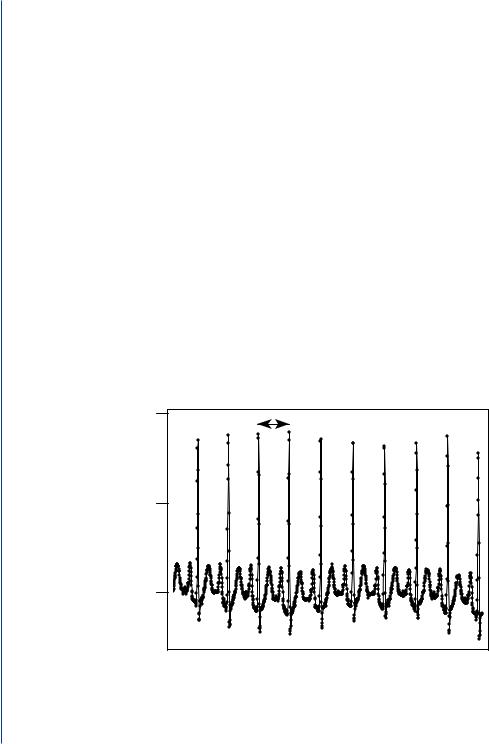
The conclusions that one may draw from using statistical analysis are only as good as the underlying model that is used to describe the real-world phenomenon, such as the time interval between heartbeats. For example, a normally functioning heart exhibits considerable variability in beat-to-beat intervals (Figure 1.1). This variability reflects the body’s continual effort to maintain homeostasis so that the body may continue to perform its most essential functions and supply the body with the oxygen and nutrients required to function normally. It has been demonstrated through biomedical research that there is a loss of heart rate variability associated with some diseases, such as diabetes and ischemic heart disease. Researchers seek to determine if this difference in variability between normal subjects and subjects with heart disease is significant (meaning, it is due to some underlying change in biology and not simply a result of chance) and whether it might be used to predict the progression of the disease [1]. One will note that the probability model changes as a consequence of changes in the underlying biological function or process. In the case of manufacturing, the probability model used to describe the output of the manufacturing process may change as
|
|
|
|
|
7,0( |
FIGURE 1.1: Example of an ECG recording, where R-R interval is defined as the time interval between successive R waves of the QRS complex, the most prominent waveform of the ECG.
introduction
a function of machine operation or changes in the surrounding manufacturing environment, such as temperature, humidity, or human operator.
Besides helping us to describe the probability model associated with real-world phenomenon, statistics help us to make decisions by giving us quantitative tools for testing hypotheses. We call this inferential statistics, whereby the outcome of a statistical test allows us to draw conclusions or make inferences about one or more populations from which samples are drawn. Most often, scientists and engineers are interested in comparing data from two or more different populations or from two or more different processes. Typically, the default hypothesis is that there is no difference in the distributions of two or more populations or processes, and we use statistical analysis to determine whether there are true differences in the distributions of the underlying populations to warrant different probability models be assigned to the individual processes.
In summary, biomedical engineers typically collect data or samples from various phenomena, which contain some element of randomness or unpredictable variability, for the purposes of making decisions. To make sound decisions in the context of the uncertainty with some level of confidence, we need to assume some probability model for the populations from which the samples have been collected. Once we have assumed an underlying model, we can select the appropriate statistical tests for comparing two or more populations and then use these tests to draw conclusions about
&ROOHFW VDPSOHV IURP D SRSXODWLRQ RU
SURFHVV
$VVXPH D SUREDELOLW\ PRGHO IRU WKH SRSXODWLRQ
(VWLPDWH SRSXODWLRQ VWDWLVWLFV IURP VDPSOH VWDWLVWLFV
&RPSDUH SRSXODWLRQV DQG WHVW K\SRWKHVHV
FIGURE 1.2: Steps in statistical analysis.

introduction to statistics for bioMEDical engineers
our hypotheses for which we collected the data in the first place. Figure 1.2 outlines the steps for performing statistical analysis of data.
In the following chapters, we will describe methods for graphically and numerically summarizing collected data. We will then talk about fitting a probability model to the collected data by briefly describing a number of well-known probability models that are used to describe biological phenomenon. Finally, once we have assumed a model for the populations from which we have collected our sample data, we will discuss the types of statistical tests that may be used to compare data from multiple populations and allow us to test hypotheses about the underlying populations.
• • • •

c h a p t e r 2
Collecting Data and
Experimental Design
Before we discuss any type of data summary and statistical analysis, it is important to recognize that the value of any statistical analysis is only as good as the data collected. Because we are using data or samples to draw conclusions about entire populations or processes, it is critical that the data collected (or samples collected) are representative of the larger, underlying population. In other words, if we are trying to determine whether men between the ages of 20 and 50 years respond positively to a drug that reduces cholesterol level, we need to carefully select the population of subjects for whom we administer the drug and take measurements. In other words, we have to have enough samples to represent the variability of the underlying population. There is a great deal of variety in the weight, height, genetic makeup, diet, exercise habits, and drug use in all men ages 20 to 50 years who may also have high cholesterol. If we are to test the effectiveness of a new drug in lowering cholesterol, we must collect enough data or samples to capture the variability of biological makeup and environment of the population that we are interested in treating with the new drug. Capturing this variability is often the greatest challenge that biomedical engineers face in collecting data and using statistics to draw meaningful conclusions. The experimentalist must ask questions such as the following:
•What type of person, object, or phenomenon do I sample?
•What variables that impact the measure or data can I control?
•How many samples do I require to capture the population variability to apply the appropriate statistics and draw meaningful conclusions?
•How do I avoid biasing the data with the experimental design?
Experimental design, although not the primary focus of this book, is the most critical step to support the statistical analysis that will lead to meaningful conclusions and hence sound decisions.
One of the most fundamental questions asked by biomedical researchers is, “What size sample do I need?” or “How many subjects will I need to make decisions with any level of confidence?”

introduction to statistics for bioMEDical engineers
We will address these important questions at the end of this book when concepts such as variability, probability models, and hypothesis testing have already been covered. For example, power tests will be described as a means for predicting the sample size required to detect significant differences in two population means using a t test.
Two elements of experimental design that are critical to prevent biasing the data or selecting samples that do not fairly represent the underlying population are randomization and blocking.
Randomization refers to the process by which we randomly select samples or experimental units from the larger underlying population such that we maximize our chance of capturing the variability in the underlying population. In other words, we do not limit our samples such that only a fraction of the characteristics or behaviors of the underlying population are captured in the samples. More importantly, we do not bias the results by artificially limiting the variability in the samples such that we alter the probability model of the sample population with respect to the probability model of the underlying population.
In addition to randomizing our selection of experimental units from which to take samples, we might also randomize our assignment of treatments to our experimental units. Or, we may randomize the order in which we take data from the experimental units. For example, if we are testing the effectiveness of two different medical imaging methods in detecting brain tumor, we will randomly assign all subjects suspect of having brain tumor to one of the two imaging methods. Thus, if we have a mix of sex, age, and type of brain tumor participating in the study, we reduce the chance of having all one sex or one age group assigned to one imaging method and a very different type of population assigned to the second imaging method. If a difference is noted in the outcome of the two imaging methods, we will not artificially introduce sex or age as a factor influencing the imaging results.
As another example, if one are testing the strength of three different materials for use in hip implants using several strength measures from a materials testing machine, one might randomize the order in which samples of the three different test materials are submitted to the machine. Machine performance can vary with time because of wear, temperature, humidity, deformation, stress, and user characteristics. If the biomedical engineer were asked to find the strongest material for an artificial hip using specific strength criteria, he or she may conduct an experiment. Let us assume that the engineer is given three boxes, with each box containing five artificial hip implants made from one of three materials: titanium, steel, and plastic. For any one box, all five implant samples are made from the same material. To test the 15 different implants for material strength, the engineer might randomize the order in which each of the 15 implants is tested in the materials testing machine so that time-dependent changes in machine performance or machine-material interactions or time-varying environmental condition do not bias the results for one or more of the materials. Thus, to fully randomize the implant testing, an engineer may literally place the numbers 1–15 in a hat and also assign the numbers 1–15 to each of the implants to be tested. The engineer will then blindly draw one of the 15 numbers from a hat and test the implant that corresponds to

collecting data and experimental design
that number. This way the engineer is not testing all of one material in any particular order, and we avoid introducing order effects into the data.
The second aspect of experimental design is blocking. In many experiments, we are interested in one or two specific factors or variables that may impact our measure or sample. However, there may be other factors that also influence our measure and confound our statistics. In good experimental design, we try to collect samples such that different treatments within the factor of interest are not biased by the differing values of the confounding factors. In other words, we should be certain that every treatment within our factor of interest is tested within each value of the confounding factor. We refer to this design as blocking by the confounding factor. For example, we may want to study weight loss as a function of three different diet pills. One confounding factor may be a person’s starting weight. Thus, in testing the effectiveness of the three pills in reducing weight, we may want to block the subjects by starting weight. Thus, we may first group the subjects by their starting weight and then test each of the diet pills within each group of starting weights.
In biomedical research, we often block by experimental unit. When this type of blocking is part of the experimental design, the experimentalist collects multiple samples of data, with each sample representing different experimental conditions, from each of the experimental units. Fig ure 2.1 provides a diagram of an experiment in which data are collected before and after patients receives therapy, and the experimental design uses blocking (left) or no blocking (right) by experimental unit. In the case of blocking, data are collected before and after therapy from the same set of human subjects. Thus, within an individual, the same biological factors that influence the biological response to the therapy are present before and after therapy. Each subject serves as his or her own control for factors that may randomly vary from subject to subject both before and after therapy. In essence, with blocking, we are eliminating biases in the differences between the two populations
Block (Repeated Measures) |
|
No Block (No repeated measures) |
|
|||||
Subject |
Measure |
Measure |
|
Subject |
Measure |
Subject |
|
Measure |
|
before |
after |
|
|
before |
|
|
after |
|
treatment |
treatment |
|
|
treatment |
|
|
treatment |
1 |
M11 |
12 |
|
1 |
M1 |
K+1 |
|
M(K+1) |
2 |
M21 |
M22 |
|
2 |
M2 |
K+2 |
|
M(K+2) |
3 |
M31 |
M32 |
|
3 |
M3 |
K+3 |
|
M(K+3) |
. |
|
|
|
. |
|
. |
|
|
. |
|
|
|
. |
|
. |
|
|
K |
MK1 |
MK2 |
|
K |
MK |
K+K |
|
M(K+K) |
FIGURE 2.1: Samples are drawn from two populations (before and after treatment), and the experimental design uses block (left) or no block (right). In this case, the block is the experimental unit (subject) from which the measures are made.

introduction to statistics for bioMEDical engineers
(before and after) that may result because we are using two different sets of experimental units. For example, if we used one set of subjects before therapy and then an entirely different set of subjects after therapy (Figure 2.1, right), there is a chance that the two sets of subjects may vary enough in sex, age, weight, race, or genetic makeup, which would lead to a difference in response to the therapy that has little to do with the underlying therapy. In other words, there may be confounding factors that contribute to the difference in the experimental outcome before and after therapy that are not only a factor of the therapy but really an artifact of differences in the distributions of the two different groups of subjects from which the two samples sets were chosen. Blocking will help to eliminate the effect of intersubject variability.
However, blocking is not always possible, given the nature of some biomedical research studies. For example, if one wanted to study the effectiveness of two different chemotherapy drugs in reducing tumor size, it is impractical to test both drugs on the same tumor mass. Thus, the two drugs are tested on different groups of individuals. The same type of design would be necessary for testing the effectiveness of weight-loss regimens.
Thus, some important concepts and definitions to keep in mind when designing experiments include the following:
•experimental unit: the item, object, or subject to which we apply the treatment and from which we take sample measurements;
•randomization: allocate the treatments randomly to the experimental units;
•blocking: assigning all treatments within a factor to every level of the blocking factor. Often, the blocking factor is the experimental unit. Note that in using blocking, we still randomize the order in which treatments are applied to each experimental unit to avoid ordering bias.
Finally, the experimentalist must always think about how representative the sample population is with respect to the greater underlying population. Because it is virtually impossible to test every member of a population or every product rolling down an assembly line, especially when destructive testing methods are used, the biomedical engineer must often collect data from a much smaller sample drawn from the larger population. It is important, if the statistics are going to lead to useful conclusions, that the sample population captures the variability of the underlying population. What is even more challenging is that we often do not have a good grasp of the variability of the underlying population, and because of expense and respect for life, we are typically limited in the number of samples we may collect in biomedical research and manufacturing. These limitations are not easy to address and require that the engineer always consider how fair the sample and data analysis is and how well it represents the underlying population(s) from which the samples are drawn.
• • • •