

54 introduction to statistics for biomedical engineers
We typically use β to denote the type II error. We will discuss this error further at the end of chapter seven when we discuss power tests.
5.2COMPARISON OF TWO VARIANCES
We used the t test to compare the means for two populations or processes. Two populations may also be compared for differences in variance. As discussed earlier, populations that are normally distributed are completely characterized by their mean and variance. Thus, if we want to test for differences between two normal populations, we need only compare their two means and their two variances.
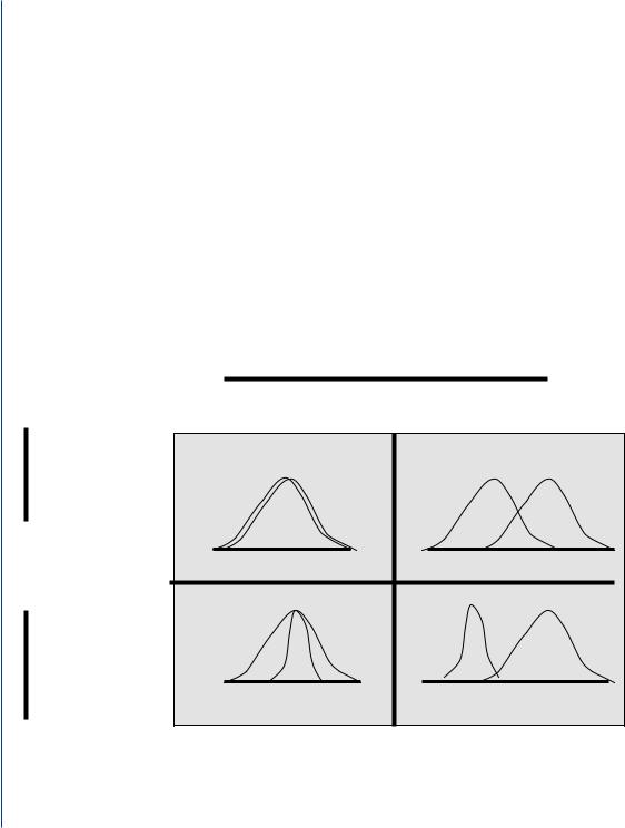
Figure 5.6 illustrates the probability density functions for two normal populations (black and red traces). The four diagrams illustrate how two different normally distributed populations may compare with each other. The right two panels differ from the left two panels in the means of the populations. The top two panels differ from the bottom two panels in variance of the populations.
t - test
Means Same |
Means Different |
Variance
Same
F - Test
Variances
Different
FIGURE 5.6: Two normal populations may differ in their means (top row), their variances (left half), or both (bottom right corner). t and F tests may be used to test for significant differences in the population means and population variances, respectively.
Statistical Inference 55
As indicated across the top of the tracings, a t test is used to test for differences in mean between the two populations. As indicated along the vertical direction, an F test is used to test for significant differences in the variances of the populations. Note that two normal populations may differ significantly in both mean and variance.
To compare the variances of two populations, we use what is referred to as an F test. As for the t test, the F test assumes that the data consist of independent random samples from each of two normal populations. If the two populations are not normally distributed, the results of the F test may be meaningless.
Frequency
F Distribution (f 10, 8)
3000
2000
1000
0
0 |
10 |
20 |
Normalized Measure
F Distribution (f 40,30)
1000
Frequency
500
0
0 |
1 |
2 |
3 |
4 |
5 |
Normalized Measure
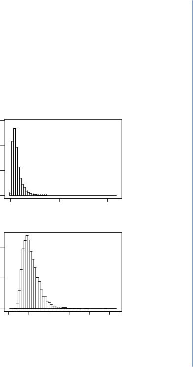
FIGURE 5.7: Histograms of samples drawn from two different F distributions. In the top panel, the two degrees of freedom are 10 and 8. In the lower panel, the two degrees of freedom are 40 and 30.

TABLE 5.1: Values from the F distribution for areas of α in the tail to the right of
F (dn, dd, α)
dn
dd |
1 |
2 |
3 |
4 |
5 |
… |
10 |
11 |
|
|
|
|
|
|
|
|
|
1 |
161, |
200, |
216, |
225, |
230, |
|
242, |
243, |
|
4052 |
4999 |
5403 |
5625 |
5764 |
|
6056 |
6082 |
|
|
|
|
|
|
|
|
|
2 |
18.51, |
19.00, |
19.16, |
|
98.49 |
99.01 |
99.17 |
3 |
10.13, |
9.55, |
9.28, |
|
34.12 |
30.81 |
29.46 |
4 |
7.71, |
6.94, |
6.59, |
|
21.20 |
18.00 |
16.69 |
5 |
6.61, |
5.79, |
5.41, |
|
16.26 |
13.27 |
12.06 |
… |
|
|
|
10 |
4.96, |
4.10, |
3.71, |
|
10.04 |
7.56 |
6.55 |
12 |
4.75, |
3.88, |
3.49, |
|
9.33 |
6.93 |
5.95 |
15 |
4.54, |
3.68, |
3.29, |
|
8.68 |
6.36 |
5.42 |
… |
|
|
|
20 |
4.35, |
3.49, |
3.10, |
|
8.10 |
5.85 |
4.94 |
50 |
4.03, |
3.18, |
2.79, |
|
7.17 |
5.06 |
4.20 |
100 |
3.94, |
3.09, |
2.70, |
|
6.90 |
4.82 |
3.98 |
200 |
3.89, |
3.04, |
2.65, |
|
6.76 |
4.71 |
3.38 |
∞ |
3.84, |
2.99, |
2.60, |
|
6.64 |
4.60 |
3.78 |
19.25, |
19.30, |
19.39, |
19.40, |
99.25 |
99.30 |
99.40 |
99.41 |
9.12, |
9.01, |
8.78, |
8.76, |
28.71 |
28.24 |
27.23 |
27.13 |
6.39, |
6.26, |
5.96, |
5.93, |
15.98 |
15.52 |
14.54 |
14.45 |
5.19, |
5.05, |
4.74, |
4.70, |
11.39 |
10.97 |
10.05 |
9.96 |
3.48, |
3.33, |
2.97, |
2.94, |
5.99 |
5.64 |
4.85 |
4.78 |
3.26, |
3.11, |
2.76, |
2.72, |
5.41 |
5.06 |
4.30 |
4.22 |
3.06, |
2.90, |
2.55, |
2.51, |
4.89 |
4.56 |
3.80 |
3.73 |
2.87, |
2.71, |
2.35, |
2.31, |
4.43 |
4.10 |
3.37 |
3.30 |
2.56, |
2.40, |
2.02, |
1.98, |
3.72 |
3.41 |
2.70 |
2.62 |
2.46, |
2.30, |
1.92, |
1.88, |
3.51 |
3.20 |
2.51 |
2.43 |
2.41, |
2.26, |
1.87, |
1.83, |
3.41 |
3.11 |
2.41 |
2.34 |
2.37, |
2.21, |
1.83, |
1.79, |
3.32 |
3.02 |
2.32 |
2.24 |
dn = degrees of freedom for numerator; dd = degrees of freedom for denominator; α = the area in distribution tail to right of F (dn, dd, α) = 0.05 or 0.01.

dn
12 |
14 |
… |
20 |
30 |
40 |
50 |
100 |
200 |
∞ |
|
|
|
|
|
|
|
|
|
|
244, |
245, |
|
248, |
250, |
251, |
252, |
253, |
254, |
254, |
6106 |
6142 |
|
6208 |
6258 |
6286 |
6302 |
6334 |
6352 |
6366 |
|
|
|
|
|
|
|
|
|
|
19.41, |
19.42, |
|
19.44, |
19.46, |
19.47, |
19.47, |
19.49, |
19.49, |
19.50, |
99.42 |
99.43 |
|
99.45 |
99.47 |
99.48 |
99.48 |
99.49 |
99.49 |
99.50 |
|
|
|
|
|
|
|
|
|
|
8.74, |
8.71, |
|
8.66, |
8.62, |
8.60, |
8.58, |
8.56, |
8.54, |
8.53, |
27.05 |
26.92 |
|
26.69 |
26.50 |
26.41 |
26.30 |
26.23 |
26.18 |
26.12 |
|
|
|
|
|
|
|
|
|
|
5.91, |
5.87, |
|
5.80, |
5.74, |
5.71, |
5.70, |
5.66, |
5.65, |
5.63, |
14.37 |
14.24 |
|
14.02 |
13.83 |
13.74 |
13.69 |
13.57 |
13.52 |
13.46 |
|
|
|
|
|
|
|
|
|
|
4.68, |
4.64, |
|
4.56, |
4.50, |
4.46, |
4.44, |
4.40, |
4.38, |
4.36, |
9.89 |
9.77 |
|
9.55 |
9.38 |
9.29 |
9.24 |
9.13 |
9.07 |
9.02 |
|
|
|
|
|
|
|
|
|
|
|
|
|
|
|
|
|
|
|
|
2.91, |
2.86, |
|
2.77, |
2.70, |
2.67, |
2.64, |
2.59, |
2.56, |
2.54, |
4.71 |
4.60 |
|
4.41 |
4.25 |
4.17 |
4.12 |
4.01 |
3.96 |
3.91 |
|
|
|
|
|
|
|
|
|
|
2.69, |
2.64, |
|
2.54, |
2.46, |
2.42, |
2.40, |
2.35, |
2.32, |
2.30, |
4.16 |
4.05 |
|
3.86 |
3.70 |
3.61 |
3.56 |
3.46 |
3.41 |
3.36 |
|
|
|
|
|
|
|
|
|
|
2.48, |
2.43, |
|
2.33, |
2.25, |
2.21, |
2.18, |
2.12, |
2.10, |
2.07, |
3.67 |
3.56 |
|
3.36 |
3.20 |
3.12 |
3.07 |
2.97 |
2.92 |
2.87 |
|
|
|
|
|
|
|
|
|
|
|
|
|
|
|
|
|
|
|
|
2.28, |
2.23, |
|
2.12, |
2.04, |
1.99, |
1.96, |
1.90, |
1.87, |
1.84, |
3.23 |
3.13 |
|
2.94 |
2.77 |
2.69 |
2.63 |
2.53 |
2.47 |
2.42 |
|
|
|
|
|
|
|
|
|
|
1.95, |
1.90, |
|
1.78, |
1.69, |
1.63, |
1.60, |
1.52, |
1.48, |
1.44, |
2.56 |
2.46 |
|
2.26 |
2.10 |
2.00 |
1.94 |
1.82 |
1.76 |
1.68 |
|
|
|
|
|
|
|
|
|
|
1.85, |
1.79, |
|
1.68, |
1.57, |
1.51, |
1.48, |
1.39, |
1.34, |
1.28, |
2.36 |
2.26 |
|
2.06 |
1.89 |
1.79 |
1.73 |
1.59 |
1.51 |
1.43 |
|
|
|
|
|
|
|
|
|
|
1.80, |
1.74, |
|
1.62, |
1.52, |
1.45, |
1.42, |
1.32, |
1.26, |
1.19, |
2.28 |
1.17 |
|
1.97 |
1.79 |
1.69 |
1.62 |
1.48 |
1.39 |
1.28 |
|
|
|
|
|
|
|
|
|
|
1.75, |
1.69, |
|
1.57, |
1.46, |
1.40, |
1.35, |
1.24, |
1.17, |
1.00, |
2.18 |
2.07 |
|
1.87 |
1.69 |
1.59 |
1.52 |
1.36 |
1.25 |
1.00 |

58 introduction to statistics for biomedical engineers
As with the t test, the F test is used to test the following hypotheses:
1.null hypothesis: H0: σ12 = σ22 and
2.alternative hypothesis: H1: σ12 > σ22,
where σ12 and σ22 are the variances of the two populations.
To reject or accept the null hypothesis, we compute the following F statistic:
F= s12 , s2 2
where s12 and s22 are the sample variance estimates of the two populations. The ratio of two variances from two normal populations is also a random variable that follows an F distribution. The F distribution is illustrated in Figure 5.7. As with the t distribution, the F distribution varies with two parameters, such as the samples sizes of the two populations. Table 5.1 shows a fraction of an F table, where two degrees of freedom, dn and dd, are required to locate an F value in the F table. In this figure, the table entries are given for significance levels (α values) of 0.05 and 0.01. The F values associated with 0.05 and 0.01 significance levels are given in regular type and boldface-italics, respectively. Thus, for any two degrees of freedom, there are two F values provided, one for the 95% confidence level and one for the 99% confidence level.
To make use of the F table with the F test, we estimate an F statistic using the sample variance estimates from each of the two populations we are trying to compare. Note that for the use of this F table, the larger of the two variances should be put in the numerator of the equation above.
We now compare our estimated F statistic to the entries in the F table associated with dn and dd degrees of freedom and appropriate confidence level (only the 95% and 99% F values are provided in the table provided). dn = n1 and dd = n2 are the number of samples in each population, with n1 being the number of samples in the population with variance placed in the numerator.
If we are to reject the null hypothesis outlined above, our calculated F statistic must be > F (α, dn, dd ) in table to reject H0 with confidence (1 – α) × 100%. The degrees of freedom, dn = n1, is the value used to locate the table entry in the horizontal direction (numerator), and dd = n2 is the degrees of freedom used to locate the table entry in the vertical direction (denominator).
Example 5.2 F test
|
Population A (n1 = 9) |
Population B (n2 = 9) |
|
|
|
Mean |
0.026 |
0.027 |
|
|
|
Variance |
2.0E − 5 |
7.4E − 5 |
|
|
|