Turing Computability

out the computation: in principle it could be completed in a finite amount of time if we stayed in good health so long, or the machine stayed in working order so long; but in practice we will die, or the machine will collapse, long before the process is complete. (There is also a worry about finding enough space to store the intermediate results of the computation, and even a worry about finding enough matter to use in writing down those results: there’s only a finite amount of paper in the world, so you’d have to writer smaller and smaller without limit; to get an infinite number of symbols down on paper, eventually you’d be trying to write on molecules, on atoms, on electrons.) But our present study will ignore these practical limitations, and work with an idealized notion of computability that goes beyond what actual people or actual machines can be sure of doing. Our eventual goal will be to prove that certain functions are not computable, even if practical limitations on time, speed, and amount of material could somehow be overcome, and for this purpose the essential requirement is that our notion of computability not be too narrow.

So far we have been sliding over a significant point. When we are given as argument a number n or pair of numbers (m, n), what we in fact are directly given is a numeral for n or an ordered pair of numerals for m and n. Likewise, if the value of the function we are trying to compute is a number, what our computations in fact end with is a numeral for that number. Now in the course of human history a great many systems of numeration have been developed, from the primitive monadic or tally notation, in which the number n is represented by a sequence of n strokes, through systems like Roman numerals, in which bunches of five, ten, fifty, one-hundred, and so forth strokes are abbreviated by special symbols, to the Hindu–Arabic or decimal notation in common use today. Does it make a difference in a definition of computability which of these many systems we adopt?

Certainly computations can be harder in practice with some notations than with others. For instance, multiplying numbers given in decimal numerals (expressing the product in the same form) is easier in practice than multiplying numbers given in something like Roman numerals. Suppose we are given two numbers, expressed in Roman numerals, say XXXIX and XLVIII, and are asked to obtain the product, also expressed in Roman numerals. Probably for most us the easiest way to do this would be first to translate from Roman to Hindu–Arabic—the rules for doing this are, or at least used to be, taught in primary school, and in any case can be looked up in reference works—obtaining 39 and 48. Next one would carry out the multiplication in our own more convenient numeral system, obtaining 1872. Finally, one would translate the result back into the inconvenient system, obtaining MDCCCLXXII. Doing all this is, of course, harder than simply performing a multiplication on numbers given by decimal numerals to begin with.

But the example shows that when a computation can be done in one notation, it is possible in principle to do in any other notation, simply by translating the data from the difficult notation into an easier one, performing the operation using the easier notation, and then translating the result back from the easier to the difficult notation. If a function is effectively computable when numbers are represented in one system of numerals, it will also be so when numbers are represented in any other system of numerals, provided only that translation between the systems can itself be

carried out according to explicit rules, which is the case for any historical system of numeration that we have been able to decipher. (To say we have been able to decipher it amounts to saying that there are rules for translating back and forth between it and the system now in common use.) For purposes of framing a rigorously defined notion of computability, it is convenient to use monadic or tally notation.

A Turing machine is a specific kind of idealized machine for carrying out computations, especially computations on positive integers represented in monadic notation. We suppose that the computation takes place on a tape, marked into squares, which is unending in both directions—either because it is actually infinite or because there is someone stationed at each end to add extra blank squares as needed. Each square either is blank, or has a stroke printed on it. (We represent the blank by S0 or 0 or most often B, and the stroke by S1 or | or most often 1, depending on the context.) And with at most a finite number of exceptions, all squares are blank, both initially and at each subsequent stage of the computation.

At each stage of the computation, the computer (that is, the human or mechanical agent doing the computation) is scanning some one square of the tape. The computer is capable of erasing a stroke in the scanned square if there is one there, or of printing a stroke if the scanned square is blank. And he, she, or it is capable of movement: one square to the right or one square to the left at a time. If you like, think of the machine quite crudely, as a box on wheels which, at any stage of the computation, is over some square of the tape. The tape is like a railroad track; the ties mark the boundaries of the squares; and the machine is like a very short car, capable of moving along the track in either direction, as in Figure 3-1.

Figure 3-1. A Turing machine.

At the bottom of the car there is a device that can read what’s written between the ties, and erase or print a stroke. The machine is designed in such a way that at each stage of the computation it is in one of a finite number of internal states, q1, . . . , qm . Being in one state or another might be a matter of having one or another cog of a certain gear uppermost, or of having the voltage at a certain terminal inside the machine at one or another of m different levels, or what have you: we are not concerned with the mechanics or the electronics of the matter. Perhaps the simplest way to picture the thing is quite crudely: inside the box there is a little man, who does all the reading and writing and erasing and moving. (The box has no bottom: the poor mug just walks along between the ties, pulling the box along.) This operator inside the machine has a list of m instructions written down on a piece of paper and is in state qi when carrying out instruction number i.

Each of the instructions has conditional form: it tells what to do, depending on whether the symbol being scanned (the symbol in the scanned square) is the blank or

stroke, S0 or S1. Namely, there are five things that can be done:

(1)Erase: write S0 in place of whatever is in the scanned square.

(2)Print: write S1 in place of whatever is in the scanned square.

(3)Move one square to the right.

(4)Move one square to the left.

(5)Halt the computation.

[In case the square is already blank, (1) amounts to doing nothing; in case the square already has a stroke in it, (2) amounts to doing nothing.] So depending on what instruction is being carried out (= what state the machine, or its operator, is in) and on what symbol is being scanned, the machine or its operator will perform one or another of these five overt acts. Unless the computation has halted (overt act number 5), the machine or its operator will perform also a covert act, in the privacy of box, namely, the act of determining what the next instruction (next state) is to be. Thus the present state and the presently scanned symbol determine what overt act is to be performed, and what the next state is to be.

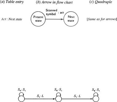
The overall program of instructions can be specified in various ways, for example, by a machine table, or by a flow chart (also called a flow graph), or by a set of quadruples. For the case of a machine that writes three symbols S1 on a blank tape and then halts, scanning the leftmost of the three, the three sorts of description are illustrated in Figure 3-2.

Figure 3-2. A Turing machine program.

3.1 Example (Writing a specified number of strokes). We indicate in Figure 3-2 a machine that will write the symbol S1 three times. A similar construction works for any specified symbol and any specified number of times. The machine will write an S1 on the square it’s initially scanning, move left one square, write an S1 there, move left one more square, write an S1 there, and halt. (It halts when it has no further instructions.) There will be three states—one for each of the symbols S1 that are to be written. In Figure 3-2, the entries in the top row of the machine table (under the horizontal line) tell the machine or its operator, when following instruction q1, that (1) an S1 is to be written and instruction q1 is to be repeated, if the scanned symbol is S0, but that (2) the machine is to move left and follow instruction q2 next, if the scanned symbol is S1. The same information is given in the flow chart by the two arrows that emerge from the node marked q1; and the same information is also given by the first two quadruples. The significance

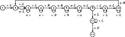
3.2 Example (Doubling the number of strokes). The machine starts off scanning the leftmost of a block of strokes on an otherwise blank tape, and winds up scanning the leftmost of a block of twice that many strokes on an otherwise blank tape. The flow chart is shown in Figure 3-5.

Figure 3-5. Doubling the number of strokes.

How does it work? In general, by writing double strokes at the left and erasing single strokes at the right. In particular, suppose the initial configuration is 1111, so that we start in state 1, scanning the leftmost of a block of three strokes on an otherwise blank tape. The next few configurations are as follows:

So we have written our first double stroke at the left—separated from the original block 111 by a blank. Next we go right, past the blank to the right-hand end of the original block, and erase the rightmost stroke. Here is how that works, in two phases. Phase 1:

Now we know that we have passed the last of the original block of strokes, so (phase 2) we back up, erase one of them, and move one more square left:

1101117 1101107 1101180.

Now we hop back left, over what is left of the original block of strokes, over the blank separating the original block from the additional strokes we have printed, and over those additional strokes, until we find the blank beyond the leftmost stroke:

Now we will print another two new strokes, much as before:

We are now back on the leftmost of the block of newly printed strokes, and the process that led to finding and erasing the rightmost stroke will be repeated, until we arrive at the following:

11110117 11110107 11110180.

Another round of this will lead first to writing another pair of strokes:

141111101.

Example 3.4. The object is to erase the leftmost stroke, fill the gap between the two blocks of strokes, and halt scanning the leftmost stroke that remains on the tape. Here is one way of doing it, in quadruple notation: q1 S1 S0q1; q1 S0Rq2; q2 S1Rq2; q2 S0 S1q3; q3 S1Lq3; q3 S0Rq4.

Example 3.5. A flow chart for a machine is shown in Figure 3-7.

Figure 3-7. Multiplication machine.

Here is how the machine works. The first block, of p strokes, is used as a counter, to keep track of how many times the machine has added q strokes to the group at the right. To start, the machine erases the leftmost of the p strokes and sees if there are any strokes left in the counter group. If not, pq = q, and all the machine has to do is position itself over the leftmost stroke on the tape, and halt.

But if there are any strokes left in the counter, the machine goes into a leapfrog routine: in effect, it moves the block of q strokes (the leapfrog group) q places to the right along the tape. For example, with p = 2 and q = 3 the tape looks like this initially:

11B111

and looks like this after going through the leapfrog routine:

B1B B B B111.

The machine will then note that there is only one 1 left in the counter, and will finish up by erasing that 1, moving right two squares, and changing all Bs to strokes until it comes to a stroke, at which point it continues to the leftmost 1 and halts.

The general picture of how the leapfrog routine works is shown in Figure 3-8.

Figure 3-8. Leapfrog.

In general, the leapfrog group consists of a block of 0 or 1 or . . . or q strokes, followed by a blank, followed by the remainder of the q strokes. The blank is there to tell the machine when the leapfrog game is over: without it the group of q strokes would keep moving right along the tape forever. (In playing leapfrog, the portion of the q strokes to the left of the blank in the leapfrog group functions as a counter: it controls the process of adding strokes to the portion of the leapfrog group to the right of the blank. That is why there are two big loops in the flow chart: one for each counter-controlled subroutine.)

We have not yet given an official definition of what it is for a numerical function to be computable by a Turing machine, specifying how inputs or arguments are to be represented on the machine, and how outputs or values represented. Our specifications for a k-place function from positive integers to positive integers are as follows:

(a)The arguments m1, . . . , mk of the function will be represented in monadic notation by blocks of those numbers of strokes, each block separated from the next by a single blank, on an otherwise blank tape. Thus, at the beginning of the computation of, say, 3 + 2, the tape will look like this: 111B11.

(b)Initially, the machine will be scanning the leftmost 1 on the tape, and will be in its initial state, state 1. Thus in the computation of 3 + 2, the initial configuration will be 1111B11. A configuration as described by (a) and (b) is called a standard initial configuration (or position).

(c)If the function that is to be computed assigns a value n to the arguments that are represented initially on the tape, then the machine will eventually halt on a tape

containing a block of that number of strokes, and otherwise blank. Thus in the computation of 3 + 2, the tape will look like this: 11111.

(d)In this case, the machine will halt scanning the leftmost 1 on the tape. Thus in the computation of 3 + 2, the final configuration will be 1n 1111, where nth state is one for which there is no instruction what to do if scanning a stroke, so that in this configuration the machine will be halted. A configuration as described by (c) and

(d)is called a standard final configuration (or position).

(e)If the function that is to be computed assigns no value to the arguments that are represented initially on the tape, then the machine either will never halt, or will halt in some nonstandard configuration such as Bn 11111 or B11n 111 or B11111n .

The restriction above to the standard position (scanning the leftmost 1) for starting and halting is inessential, but some specifications or other have to be made about initial and final positions of the machine, and the above assumptions seem especially simple.

With these specifications, any Turing machine can be seen to compute a function of one argument, a function of two arguments, and, in general, a function of k arguments for each positive integer k. Thus consider the machine specified by the single quadruple q111q2. Started in a standard initial configuration, it immediately halts, leaving the tape unaltered. If there was only a single block of strokes on the tape initially, its final configuration will be standard, and thus this machine computes the identity function id of one argument: id(m) = m for each positive integer m. Thus the machine computes a certain total function of one argument. But if there were two or more blocks of strokes on the tape initially, the final configuration will not be standard. Accordingly, the machine computes the extreme partial function of two arguments that is undefined for all pairs of arguments: the empty function e2 of two arguments. And in general, for k arguments, this machine computes the empty function ek of k arguments.

Figure 3-9. A machine computing the value 1 for all arguments.

By contrast, consider the machine whose flow chart is shown in Figure 3-9. This machine computes for each k the total function that assigns the same value, namely 1, to each k-tuple. Started in initial state 1 in a standard initial configuration, this machine erases the first block of strokes (cycling between states 1 and 2 to do so) and goes to state 3, scanning the second square to the right of the first block. If it sees a blank there, it knows it has erased the whole tape, and so prints a single 1 and halts in state 4, in a standard configuration. If it sees a stroke there, it re-enters the cycle between states 1 and 2, erasing the second block of strokes and inquiring again, in state 3, whether the whole tape is blank, or whether there are still more blocks to be dealt with.

A numerical function of k arguments is Turing computable if there is some Turing machine that computes it in the sense we have just been specifying. Now computation in the Turing-machine sense is certainly one kind of computation in the intuitive sense, so all Turing-computable functions are effectively computable. Turing’s thesis is that, conversely, any effectively computable function is Turing computable, so that computation in the precise technical sense we have been developing coincides with effective computability in the intuitive sense.

It is easy to imagine liberalizations of the notion of the Turing machine. One could allow machines using more symbols than just the blank and the stroke. One could allow machines operating on a rectangular grid, able to move up or down a square as well as left or right. Turing’s thesis implies that no liberalization of the notion of Turing machine will enlarge the class of functions computable, because all functions that are effectively computable in any way at all are already computable by a Turing machine of the restricted kind we have been considering. Turing’s thesis is thus a bold claim.

It is possible to give a heuristic argument for it. After all, effective computation consists of moving around and writing and perhaps erasing symbols, according to definite, explicit rules; and surely writing and erasing symbols can be done stroke by stroke, and moving from one place to another can be done step by step. But the main argument will be the accumulation of examples of effectively computable functions that we succeed in showing are Turing computable. So far, however, we have had just a few examples of Turing machines computing numerical functions, that is, of effectively computable functions that we have proved to be Turing computable: addition and multiplication in the preceding section, and just now the identity function, the empty function, and the function with constant value 1.

Now addition and multiplication are just the first two of a series of arithmetic operations all of which are effectively computable. The next item in the series is exponentiation. Just as multiplication is repeated addition, so exponentiation is repeated multiplication. (Then repeated exponentiation gives a kind of super-exponentiation, and so on. We will investigate this general process of defining new functions from old in a later chapter.) If Turing’s thesis is correct, there must be a Turing machine for each of these functions, computing it. Designing a multiplier was already difficult enough to suggest that designing an exponentiator would be quite a challenge, and in any case, the direct approach of designing a machine for each operation would take us forever, since there are infinitely many operations in the series. Moreover, there are many other effectively computable numerical functions besides the ones in this series. When we return, in the chapter after next, to the task of showing various effectively computable numerical functions to be Turing computable, and thus accumulating evidence for Turing’s thesis, a less direct approach will be adopted, and all the operations in the series that begins with addition and multiplication will be shown to be Turing computable in one go.

For the moment, we set aside the positive task of showing functions to be Turing computable and instead turn to examples of numerical functions of one argument that are Turing uncomputable (and so, if Turing’s thesis is correct, effectively uncomputable).