

5
Abacus Computability
Showing that a function is Turing computable directly, by giving a table or flow chart for a Turing machine computing the function, is rather laborious, and in the preceding chapters we did not get beyond showing that addition and multiplication and a few other functions are Turing computable. In this chapter we provide a less direct way of showing functions to be Turing computable. In section 5.1 we introduce an ostensibly more flexible kind of idealized machine, an abacus machine, or simply an abacus. In section 5.2 we show that despite the ostensible greater flexibility of these machines, in fact anything that can be computed on an abacus can be computed on a Turing machine. In section 5.3 we use the flexibility of these machines to show that a large class of functions, including not only addition and multiplication, but exponentiation and many other functions, are computable on a abacus. In the next chapter functions of this class will be called recursive, so what will have been proved by the end of this chapter is that all recursive functions are Turing computable.
5.1 Abacus Machines
We have shown addition and multiplication to be Turing-computable functions, but not much beyond that. Actually, the situation is even a bit worse. It seemed appropriate, when considering Turing machines, to define Turing computability for functions on positive integers (excluding zero), but in fact it is customary in work on other approaches to computability to consider functions on natural numbers (including zero). If we are to compare the Turing approach with others, we must adapt our definition of Turing computability to apply to natural numbers, as can be accomplished (at the cost of some slight artificiality) by the expedient of letting the number n be represented by a string of n + 1 strokes, so that a single stroke now represents zero, two strokes represent one, and so on. But with this change, the adder we presented in the last chapter actually computes m + n + 1, rather than m + n, and would need to be modified to compute the standard addition function; and similarly for the multiplier. The modifications are not terribly difficult to carry out, but they still leave us with only a very few examples of interesting effectively computable functions that have been shown to be Turing computable. In this chapter we greatly enlarge the number of examples, but we do not do so directly, by giving tables or flow charts for the relevant Turing machines. Instead, we do so indirectly, by way of another kind of idealized machine.
45
46 |
ABACUS COMPUTABILITY |
Historically, the notion of Turing computability was developed before the age of high-speed digital computers, and in fact, the theory of Turing computability formed a not insignificant part of the theoretical background for the development of such computers. The kinds of computers that are ordinary today are in one respect more flexible than Turing machines in that they have random-access storage. A Lambek or abacus machine or simply abacus will be an idealized version of computer with this ‘ordinary’ feature. In contrast to a Turing machine, which stores information symbol by symbol on squares of a one-dimensional tape along which it can move a single step at a time, a machine of the seemingly more powerful ‘ordinary’ sort has access to an unlimited number of registers R0, R1, R2, . . . , in each of which can be written numbers of arbitrary size. Moreover, this sort of machine can go directly to register Rn without inching its way, square by square, along the tape. That is, each register has its own address (for register Rn it might be just the number n) which allows the machine to carry out such instructions as
put the sum of the numbers in registers Rm and Rn into register Rp
which we abbreviate
[m] + [n] → p.
In general, [n] is the number in register Rn , and the number at the right of an arrow identifies the register in which the result of the operation at the left of the arrow is to be stored. When working with such machines, it is natural to consider functions on the natural numbers (including zero), and not just the positive integers (excluding zero). Thus, the number [n] in register Rn at a given time may well be zero: the register may be empty.
It should be noted that our ‘ordinary’ sort of computing machine is really quite extraordinary in one respect: although real digital computing machines often have random-access storage, there is always a finite upper limit on the size of the numbers that can be stored; for example, a real machine might have the ability to store any of the numbers 0, 1, . . . , 10 000 000 in each of its registers, but no number greater than ten million. Thus, it is entirely possible that a function that is computable in principle by one of our idealized machines is not computable in practice by any real machine, simply because, for certain arguments, the computation would require more capacious registers than any real machine possesses. (Indeed, addition is a case in point: there is no finite bound on the sizes of the numbers one might think of adding, and hence no finite bound on the size of the registers needed for the arguments and the sum.) But this is in line with our objective of abstracting from technological limitations so as to arrive at a notion of computability that is not too narrow. We seek to show that certain functions are uncomputable in an absolute sense: uncomputable even by our idealized machines, and therefore uncomputable by any past, present, or future real machine.
In order to avoid discussion of electronic or mechanical details, we may imagine the abacus machine in crude, Stone Age terms. Each register may be thought of as a roomy, numbered box capable of holding any number of stones: none or one or two or . . . , so that [n] will be the number of stones in box number n. The ‘machine’ can
5.1. ABACUS MACHINES |
47 |
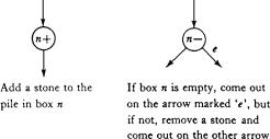
be thought of as operated by a little man who is capable of carrying out two sorts of operations: adding a stone to the box of a specified number, and removing a stone from the box of a specified number, if there are any stones there to be removed.
The table for a Turing machine is in effect a list of numbered instructions, where ‘attending to instruction q’ is called ‘being in state q’. The instructions all have the following form:
(q) |
if you are scanning a blank |
then perform action a and go to r |
|
if you are scanning a stroke |
then perform action b and go to s. |
||
|
Here each of the actions is one of the following four options: erase (put a blank in the scanned square), print (put a stroke in the scanned square), move left, move right. It is permitted that one or both of r or s should be q, so ‘go to r’ or ‘go to s’ amounts to ‘remain with q’.
Turing machines can also be represented by flow charts, in which the states or instructions do not have to be numbered. An abacus machine program could also be represented in a table of numbered instructions. These would each be of one or the other of the following two forms:
(q) |
add one to box m and go to r |
||
(q) |
if box m is not empty |
then subtract one from box m and go to r |
|
if box m is empty |
then go to s. |
||
|
|||
But in practice we are going to be working throughout with a flow-chart representation. In this representation, the elementary operations will be symbolized as in Figure 5-1.
Figure 5-1. Elementary operations in abacus machines.
Flow charts can be built up as in the following examples.
5.1 Example (Emptying box n). Emptying the box of a specified number n can be accomplished with a single instruction as follows:
(1)
if box n is not empty if box n is empty
then subtract 1 from box n and stay with 1 then halt.
The corresponding flow chart is indicated in Figure 5-2.
In the figure, halting is indicated by an arrow leading nowhere. The block diagram also shown in Figure 5-2 summarizes what the program shown in the flow chart accomplishes,
48 |
ABACUS COMPUTABILITY |
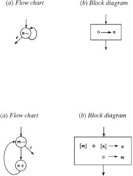
Figure 5-2. Emptying a box.
without indicating how it is accomplished. Such summaries are useful in showing how more complicated programs can be put together out of simpler ones.
5.2 Example (Emptying box m into box n). The program is indicated in Figure 5-3.
Figure 5-3. Emptying one box into another.
The figure is intended for the case m = n. (If m = n, the program halts—exits on the e arrow—either at once or never, according as the box is empty or not originally.) In future we assume, unless the contrary possibility is explicitly allowed, that when we write of boxes m, n, p, and so on, distinct letters represent distinct boxes.
When as intended m = n, the effect of the program is the same as that of carrying stones from box m to box n until box m is empty, but there is no way of instructing the machine or its operator to do exactly that. What the operator can do is (m−) take stones out of box m, one at a time, and throw them on the ground (or take them to wherever unused stones are stored), and then (n+) pick stones up off the ground (or take them from wherever unused stones are stored) and put them, one at a time, into box n. There is no assurance that the stones put into box n are the very same stones that were taken out of box m, but we need no such assurance in order to be assured of the desired effect as described in the block diagram, namely,
[m] + [n] → n: the number of stones in box n after this move equals the sum of the numbers in m and in n before the move
and then
0 → m: the number of stones in box m after this move is 0.
5.3 Example (Adding box m to box n, without loss from m). To accomplish this we must make use of an auxiliary register p, which must be empty to begin with (and will be empty again at the end as well). Then the program is as indicated in Figure 5-4.

5.1. ABACUS MACHINES |
49 |
Figure 5-4. Addition.
In case no assumption is made about the contents of register p at the beginning, the operation accomplished by this program is the following:
[m] + [n] → n
[m] + [ p] → m
0 → p.
Here, as always, the vertical order represents a sequence of moves, from top to bottom. Thus, p is emptied after the other two moves are made. (The order of the first two moves is arbitrary: The effect would be the same if their order were reversed.)
5.4 Example (Multiplication). The numbers to be multiplied are in distinct boxes m1 and m2; two other boxes, n and p, are empty to begin with. The product appears in box n. The program is indicated in Figure 5-5.
Figure 5-5. Multiplication.
Instead of constructing a flow chart de novo, we use the block diagram of the preceding example a shorthand for the flow chart of that example. It is then straightforward to draw the full flow chart, as in Figure 5-5(b), where the m of the preceding example is changed to m2. The procedure is to dump [m2] stones repeatedly into box n, using box m1 as a counter:
50 |
ABACUS COMPUTABILITY |
We remove a stone from box m1 before each dumping operation, so that when box m1 is empty we have
[m2] + [m2] + · · · + [m2] ([m1] summands)
stones in box n.
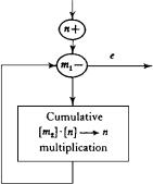
5.5 Example (Exponentiation). Just as multiplication is repeated addition, so exponentiation is repeated multiplication. The program is perfectly straightforward, once we arrange the multiplication program of the preceding example to have [m2] · [n] → n. How that is to be accomplished is shown in Figure 5-6.
Figure 5-6. Exponentiation.
The cumulative multiplication indicated in this abbreviated flow chart is carried out in two steps. First, use a program like Example 5.4 with a new auxiliary:
[n] · [m2] → q 0 → n.
Second, use a program like Example 5.2:
[q] + [n] → n
0 → q.
The result gives [n] · [m2] → n. Provided the boxes n, p, and q are empty initially, the program for exponentiation has the effect
[m2][m1] → n
0 → m1
in strict analogy to the program for multiplication. (Compare the diagrams in the preceding example and in this one.)
Structurally, the abbreviated flow charts for multiplication and exponentiation differ only in that for exponentiation we need to put a single stone in box n at the beginning. If [m1] = 0 we have n = 1 when the program terminates (as it will at once, without going through the multiplication routine). This corresponds to the convention that x0 = 1 for any natural number x. But if [m1] is positive, [n] will finally be a product of [m1] factors [m2], corresponding to repeated application of