


86 |
RECURSIVE SETS AND RELATIONS |
so if yi = gi (x1, . . . , xn ), then where y is the largest of the yi , we have y < x + a. And so
h(x1, . . . , xn ) = f (y1, . . . , ym ) < (x + a) + b = x + (a + b) and we may take c = a + b.
Problems
7.1Let R be a two-place primitive recursive, recursive, or semirecursive relation. Show that the following relations are also primitive recursive, recursive, or semirecursive, accordingly:
(a)the converse of R, given by S(x, y) ↔ R(y, x)
(b)the diagonal of R, given by D(x) ↔ R(x, x)
(c)for any natural number m, the vertical and horizontal sections of R at m, given by
Rm (y) ↔ R(m, y) and Rm (x) ↔ R(x, m).
7.2Prove that the function lg of Example 7.11 is, as there asserted, primitive recursive.
7.3For natural numbers, write u | v to mean that u divides v without remainder, that is, there is a w such that u · w = v. [Thus u | 0 holds for all u, but 0 | v holds only for v = 0.] We say z is the greatest common divisor of x and y, and write z = gcd(x, y), if z | x and z | y and whenever w | x and w | y, then w ≤ z [except that, by convention, we let gcd(0, 0) = 0]. We say z is the least common
multiple of x and y, and write z = lcm(x, y), if x | z and y | z and whenever x |w and y |w, then z ≤ w. Show that the functions gcd and lcm are primitive recursive.
7.4For natural numbers, we say x and y are relatively prime if gcd(x, y) = 1, where gcd is as in the preceding problem. The Euler φ-function φ(n) is defined as the number of m < n such that gcd(m, n) = 1. Show that φ is primitive recursive. More generally, let Rx y be a (primitive) recursive relation, and let r(x) = the number of y < x such that Rx y. Show that r is (primitive) recursive.
7.5Let A be an infinite recursive set, and for each n, let a(n) be the nth element of A in increasing order (counting the least element as the 0th). Show that the function a is recursive.
7.6Let f be a (primitive) recursive total function, and let A be the set of all n such that the value f (n) is ‘new’ in the sense of being different from f (m) for all m < n. Show that A is (primitive) recursive.
7.7Let f be a recursive total function whose range is infinite. Show that there is a one-to-one recursive total function g whose range is the same as that of f .
7.8Let us define a real number ξ to be primitive recursive if the function f (x) = the
digit in the (x + 1)st place in the decimal expansion of ξ is primitive recursive.
√
[Thus if ξ = 2 = 1.4142 . . . , then f (0) = 4, f (1) = 1, f (2) = 4, f (3) = 2,
√
and so on.] Show that 2 is a primitive recursive real number.
PROBLEMS |
87 |
7.9Let f (n) be the nth entry in the infinite sequence 1, 1, 2, 3, 5, 8, 13, 21,
. . . of Fibonacci numbers. Then f is determined by the conditions f (0) = f (1) = 1, and f (n+ 2) = f (n) + f (n + 1). Show that f is a primitive recursive function.
7.10Show that the truncation function of Example 7.21 is primitive recursive.
7.11Show that the substitution function of Example 7.22 is primitive recursive.
The remaining problems pertain to Example 7.23 in the optional section 7.3. If you are not at home with the method of proof by mathematical induction, you should probably defer these problems until after that method has been discussed in a later chapter.
7.12If f and g are n- (and n + 2)-place primitive recursive functions obtainable from the initial functions (zero, successor, identity) by composition, without use of recursion, we have shown in Proposition 7.24 that there are numbers a and b such that for all x1, . . . , xn , y, and z we have
f (x1, . . . , xn ) < x + a, where x is the largest of x1, . . . , xn
g(x1, . . . , xn , y, z) < x + b, where x is the largest of x1, . . . , xn , y, and z.
Show now that if h = Pr[ f , g], then there is a number c such that for all x1, . . . , xn and y we have
h(x1, . . . , xn , y) < cx + c, where x is the largest of x1, . . . , xn and y.
7.13Show that if f and g1, . . . , gm are functions with the property ascribed to the function h in the preceding problem, and if j = Cn[ f , g1, . . . , gm ], then j also has that property.
7.14Show that the multiplication or product function is not obtainable from the initial functions by composition without using recursion at least twice.
7.15Let β be the function considered in Example 7.23. Consider a natural number s that codes a sequence (s0, . . . , sm ) whose every entry si is itself a code for a sequence (bi,0, . . . , bi,ni ). Call such an s a β-code if the following conditions are met:
if i < m, then bi,0 = 2
if j < n0, then b0, j+1 = b0, j
if i < m and j < ni+1, then c = bi+1, j ≤ ni and bi+1, j+1 = bi,c. Call such an s a β-code covering ( p, q) if p ≤ m and q ≤ n p.
(a)Show that if s is a β-code covering ( p, q), then bp,q = β( p, q).
(b)Show that for every p it is the case that for every q there exists a β-code covering ( p, q).
7.16Continuing the preceding problem, show that the relation Rspqx, which we define to hold if and only if s is a β-code covering ( p, q) and bp,q = x, is a primitive recursive relation.
7.17Continuing the preceding problem, show that β is a recursive (total) function.
8
Equivalent Definitions of Computability
In the preceding several chapters we have introduced the intuitive notion of effective computability, and studied three rigorously defined technical notions of computability: Turing computability, abacus computability, and recursive computability, noting along the way that any function that is computable in any of these technical senses is computable in the intuitive sense. We have also proved that all recursive functions are abacus computable and that all abacus-computable functions are Turing computable. In this chapter we close the circle by showing that all Turing-computable functions are recursive, so that all three notions of computability are equivalent. It immediately follows that Turing’s thesis, claiming that all effectively computable functions are Turing computable, is equivalent to Church’s thesis, claiming that all effectively computable functions are recursive. The equivalence of these two theses, originally advanced independently of each other, does not amount to a rigorous proof of either, but is surely important evidence in favor of both. The proof of the recursiveness of Turing-computable functions occupies section 8.1. Some consequences of the proof of equivalence of the three notions of computability are pointed out in section 8.2, the most important being the existence of a universal Turing machine, a Turing machine capable of simulating the behavior of any other Turing machine desired. The optional section 8.3 rounds out the theory of computability by collecting basic facts about recursively enumerable sets, sets of natural numbers that can be enumerated by a recursive function. Perhaps the most basic fact about them is that they coincide with the semirecursive sets introduced in the preceding chapter, and hence, if Church’s (or equivalently, Turing’s) thesis is correct, coincide with the (positively) effectively semidecidable sets.
8.1 Coding Turing Computations
At the end of Chapter 5 we proved that all abacus-computable functions are Turing computable, and that all recursive functions are abacus computable. (To be quite accurate, the proofs given for Theorem 5.8 did not consider the three processes in their most general form. For instance, we considered only the composition of a twoplace function f with two three-place functions g1 and g2. But the methods of proof used were perfectly general, and do suffice to show that any recursive function can be computed by some Turing machine.) Now we wish to close the circle by proving, conversely, that every function that can be computed by a Turing machine is recursive.
We will concentrate on the case of a one-place Turing-computable function, though our argument readily generalizes. Let us suppose, then, that f is a one-place function
88
8.1. CODING TURING COMPUTATIONS |
89 |
computed by a Turing machine M. Let x be an arbitrary natural number. At the beginning of its computation of f (x), M’s tape will be completely blank except for a block of x + 1 strokes, representing the argument or input x. At the outset M is scanning the leftmost stroke in the block. When it halts, it is scanning the leftmost stroke in a block of f (x) + 1 strokes on an otherwise completely blank tape, representing the value or output f (x). And throughout the computation there are finitely many strokes to the left of the scanned square, finitely many strokes to the right, and at most one stroke in the scanned square. Thus at any time during the computation, if there is a stroke to the left of the scanned square, there is a leftmost stroke to the left, and similarly for the right. We wish to use numbers to code a description of the contents of the tape. A particularly elegant way to do so is through the Wang coding. We use binary notation to represent the contents of the tape and the scanned square by means of a pair of natural numbers, in the following manner:
If we think of the blanks as zeros and the strokes as ones, then the infinite portion of the tape to the left of the scanned square can be thought of as containing a binary numeral (for example, 1011, or 1, or 0) prefixed by an infinite sequence of superfluous 0s. We call this numeral the left numeral, and the number it denotes in binary notation the left number. The rest of the tape, consisting of the scanned square and the portion to its right, can be thought of as containing a binary numeral written backwards, to which an infinite sequence of superfluous 0s is attached. We call this numeral, which appears backwards on the tape, the right numeral, and the number it denotes the right number. Thus the scanned square contains the digit in the unit’s place of the right numeral. We take the right numeral to be written backwards to insure that changes on the tape will always take place in the vicinity of the unit’s place of both numerals. If the tape is completely blank, then the left numeral = the right numeral = 0, and the left number = the right number = 0.
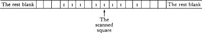
8.1 Example (The Wang coding). Suppose the tape looks as in Figure 8-1. Then the left numeral is 11101, the right numeral is 10111, the left number is 29, and the right number is 23. M now moves left, then the new left numeral is 1110, and the new left number is 14, while the new right numeral is 101111, and the new right number is 47.
Figure 8-1. A Turing machine tape to be coded.
What are the left and right numbers when M begins the computation? The tape is then completely blank to the left of the scanned square, and so the left numeral is 0 and the left number is 0. The right numeral is 11 . . . 1, a block of x + 1 digits 1. A sequence of m strokes represents in binary notation
2m−1 + · · · + 22 + 2 + 1 = 2m − 1.
90 |
EQUIVALENT DEFINITIONS OF COMPUTABILITY |
Thus the right number at the start of M’s computation of f (x) will be
strt(x) |
= |
2(x+1) |
. |
1. |
|
|
− |
|
Note that strt is a primitive recursive function.
How do the left and right numbers change when M performs one step in the computation? That depends, of course, on what symbol is being scanned, as well as on what act is performed. How can we determine the symbol scanned? It will be a blank, or 0, if the binary representation of the right number ends in a 0, as is the case when the number is even, and a stroke, or 1, if the binary representation of the right number ends in a 1, as is the case when the number is odd. Thus in either case it will be the remainder on dividing the right number by two, or in other words, if the right number is r, then the symbol scanned will be
scan(r) = rem(r, 2).
Note that scan is a primitive recursive function.
Suppose the act is to erase, or put a 0 on, the scanned square. If there was already a 0 present, that is, if scan(r) = 0, there will be no change in the left or right number. If there was a 1 present, that is, if scan(r) = 1, the left number will be unchanged, but the right number will be decreased by 1. Thus if the original left and right numbers were p and r respectively, then the new left and new right numbers will be given by
newleft0( p, r) = p
newrght ( , ) . scan( ).
0 p r = r − r
If instead the act is to print, or put a 1 on, the scanned square, there will again be no change in the left number, and there will be no change in the right number either if there was a 1 present. But if there was a 0 present, then the right number will be increased by 1. Thus the new left and new right number will be given by
newleft1( p, r) = p
newrght ( , ) 1 . scan( ).
1 p r = r + − r
Note that all the functions here are primitive recursive.
What happens when M moves left or right? Let p and r be the old (pre-move) left and right numbers, and let p* and r* be the new (post-move) left and right numbers. We want to see how p* and r* depend upon p, r, and the direction of the move. We consider the case where the machine moves left.
If p is odd, the old numeral ends in a one. If r = 0, then the new right numeral is 1, and r* = 1 = 2r + 1. And if r > 0, then the new right numeral is obtained from the old by appending a 1 to it at its one’s-place end (thus lengthening the numeral); again r* = 2r + 1. As for p*, if p = 1, then the old left numeral is just 1, the new left numeral is 0, and p* = 0 = ( p −˙ 1)/2 = quo( p, 2). And if p is any odd number greater than 1, then the new left numeral is obtained from the old by deleting
the 1 in its one’s place (thus shortening the numeral), and again * ( . 1)/2
p = p − = quo( p, 2). [In Example 8.1, for instance, we had p = 29, p* = (29 − 1)/2 = 14,
8.1. CODING TURING COMPUTATIONS |
91 |
r = 23, r* = 2 · 23 + 1 = 47.] Thus we have established the first of the following two claims:
If M moves left |
and p is odd |
then p* = quo(p, 2) |
and r* = 2r + 1 |
If M moves left |
and p is even |
then p* = quo(p, 2) |
and r* = 2r. |
The second claim is established in exactly the same way, and the two claims may be subsumed under the single statement that when M moves left, the new left and right numbers are given by
newleft2( p, r) = quo( p, 2) newrght2( p, r) = 2r + rem( p, 2).
A similar analysis shows that if M moves right, then the new left and right numbers are given by
newleft3( p, r) = 2 p + rem(r, 2) newrght3( p, r) = quo(r, 2).
Again all the functions involved are primitive recursive. If we call printing 0, printing 1, moving left, and moving right acts numbers 0, 1, 2, and 3, then the new left number when the old left and right numbers are p and r and the act number is a will be given by
p |
if a = 0 |
or a = 1 |
newleft( p, r, a) = quo( p, 2) |
if a = 2 |
|
2 p + rem(r, 2) |
if a = 3. |
|
This again is a primitive recursive function, and there is a similar primitive recursive function newrght( p, r, a) giving the new right number in terms of the old left and right numbers and the act number.
And what are the left and right numbers when M halts? If M halts in standard position (or configuration), then the left number must be 0, and the right number must
f (x)+1 . 1, which is the number denoted in binary notation by a string of be r = 2 −
f (x) + 1 digits 1. Then f (x) will be given by
valu(r) = lg(r, 2).
Here lg is the primitive recursive function of Example 7.11, so valu is also primitive recursive. If we let nstd be the characteristic function of the relation
p = 0 r = 2 |
lg(r, 2) |
+ − 1 |
|
1 . |
then the machine will be in standard position if and only if nstd( p, r) = 0. Again, since the relation indicated is primitive recursive, so is the function nstd.
So much, for the moment, for the topic of coding the contents of a Turing tape. Let us turn to the coding of Turing machines and their operations. We discussed the coding of Turing machines in section 4.1, but there we were working with positive integers and here we are working with natural numbers, so a couple of changes will be in order. One of these has already been indicated: we now number the acts 0 through 3 (rather than 1 through 4). The other is equally simple: let us now use
92 |
EQUIVALENT DEFINITIONS OF COMPUTABILITY |
0 for the halted state. A Turing machine will then be coded by a finite sequence whose length is a multiple of four, namely 4k, where k is the number of states of the machine (not counting the halted state), and with the even-numbered entries (starting with the initial entry, which we count as entry number 0) being numbers ≤3 to represent possible acts, while the odd-numbered entries are numbers ≤ k, representing possible states. Or rather, a machine will be coded by a number coding such a finite sequence.
The instruction as to what act to perform when in state q and scanning symbol i
will be given by entry number 4(q . 1) 2i, and the instruction as to what state to
− +
go into will be given by entry number 4( . 1) 2 1. For example, the 0th entry q − + i +
tells what act to perform if in the initial state 1 and scanning a blank 0, and the 1st entry what state then to go into; while the 2nd entry tells what act to perform if in initial state 1 and scanning a stroke 1, and the 3rd entry what state then to go into. If the machine with code number m is in state q and the right number is r, so that the symbol being scanned is, as we have seen, given by scan(r), then the next action to be performed and new state to go into will be given by
actn(m, q, r) newstat(m, q, r)
ent( , 4( . 1) 2 scan( ))
= m q − + · r
ent( , (4( . 1) 2 scan( )) 1).
= m q − + · r +
These are primitive recursive functions.
We have discussed representing the tape contents at a given stage of computation by two numbers p and r. To represent the configuration at a given stage of computation, we need also to mention the state q the machine is in. The configuration is then represented by a triple ( p, q, r), or by a single number coding such a triple. For definiteness let us use the coding
trpl( p, q, r) = 2p3q 5r .
Then given a code c for the configuration of the machine, we can recover the left, state, and right numbers by
left(c) = lo(c, 2) |
stat(c) = lo(c, 3) |
rght(c) = lo(c, 5) |
where lo is the primitive recursive function of Example 7.11. Again all the functions here are primitive recursive.
Our next main goal will be to define a primitive recursive function conf(m, x, t) that will give the code for the configuration after t stages of computation when the machine with code number m is started with input x, that is, is started in its initial state 1 on the leftmost of a block of x + 1 strokes on an otherwise blank tape. It should be clear already what the code for the configuration will be at the beginning, that is, after 0 stages of computation. It will be given by
inpt(m, x) = trpl(0, 1, strt(x)).
What we need to analyse is how to get from a code for the configuration at time t to the configuration at time t = t + 1.
Given the code number m for a machine and the code number c for the configuration at time t, to obtain the code number c* for the configuration at time t + 1, we may
8.1. CODING TURING COMPUTATIONS |
93 |
proceed as follows. First, apply left, stat, and rght to c to obtain the left number, state number, and right number p, q, and r. Then apply actn and newstat to m and r to obtain the number a of the action to be performed, and the number q* of the state then to enter. Then apply newleft and newrght to p, r, and a to obtain the new left and right numbers p* and r*. Finally, apply trpl to p*, q*, and r* to obtain the desired c*, which is thus given by
c* = newconf(m, c)
where newconf is a composition of the functions left, stat, rght, actn, newstat, newleft, newrght, and trpl, and is therefore a primitive recursive function.
The function conf(m, x, t), giving the code for the configuration after t stages of computation, can then be defined by primitive recursion as follows:
conf (m, x, 0) = inpt(m, x)
conf (m, x, t ) = newconf (m, conf(m, x, t)).
It follows that conf is itself a primitive recursive function.
The machine will be halted when stat(conf(m, x, t)) = 0, and will then be halted in standard position if and only if nstd(conf(m, x, t)) = 0. Thus the machine will be halted in standard position if and only if stdh(m, x, t) = 0, where
stdh(m, x, t) = stat(conf(m, x, t)) + nstd(conf(m, x, t)).
If the machine halts in standard configuration at time t, then the output of the machine will be given by
otpt(m, x, t) = valu(rght(conf(m, x, t))).
Note that stdh and otpt are both primitive recursive functions.
The time (if any) when the machine halts in standard configuration will be given by
halt(m, x) |
= |
the least t such that stdh(m, x, t) = 0 |
if such a t exists |
|
undefined |
otherwise. |
This function, being obtained by minimization from a primitive recursive function, is a recursive partial or total function.
Putting everything together, let F(m, x) = otpt(m, x, halt(m, x)), a recursive function. Then F(m, x) will be the value of the function computed by the Turing machine with code number m for argument x, if that function is defined for that argument, and will be undefined otherwise. If f is a Turing-computable function, then for some m—namely, for the code number of any Turing machine computing f —we have f (x) = F(m, x) for all x. Since F is recursive, it follows that f is recursive. We have proved:
8.2 Theorem. A function is recursive if and only if it is Turing computable.
The circle is closed.