Добавил:

fench Опубликованный материал нарушает ваши авторские права? Сообщите нам.

Вуз:

Сумский государственный педагогический университет им. Макаренко

Предмет:

Теория вероятностей и математическая статистика

Файл:

Теория информации / Cover T.M., Thomas J.A. Elements of Information Theory. 2006., 748p

.pdf

Скачиваний:

239

Добавлен:

09.08.2013

Размер:

10.58 Mб

Скачать

☆

<<< < Предыдущая 54 55 56 57 58 59 60 61 62 63 64 65 66 67 6869 / 7869 70 71 72 73 74 75 76 77 78 > Следующая >>>

			HISTORICAL NOTES 655
	1
bˆ 2	(x1) =	0 1bS1(b) db		.
	0		S1(b) db

ˆ ˆ

(f)Which of S2(b), S2 , S2, b2 are unchanged if we permute the order of appearance of the stock vector outcomes [i.e., if the sequence is now (1, 2), (1, 12 )]?

16.10Growth optimal . Let X1, X2 ≥ 0, be price relatives of two independent stocks. Suppose that EX1 > EX2. Do you always want some of X1 in a growth rate optimal portfolio S(b) = bX1 + bX2? Prove or provide a counterexample.

16.11Cost of universality . In the discussion of ﬁnite-horizon universal portfolios, it was shown that the loss factor due to universality is

1	n n	k	k	n − k	n−k .	(16.233)

Vn	= k n			n
	k=0

Evaluate Vn for n = 1, 2, 3.

16.12Convex families. This problem generalizes Theorem 16.2.2. We

say that S is a convex family of random variables if S1, S2 S

implies that λS1 + (1 − λ)S2 S. Let S be a closed convex family of random variables. Show that there is a random variable S S such that

E ln ≤ 0 (16.234)

for all S S if and only if

E ≤ 1 (16.235)

for all S S.

HISTORICAL NOTES

There is an extensive literature on the mean – variance approach to investment in the stock market. A good introduction is the book by Sharpe [491]. Log-optimal portfolios were introduced by Kelly [308] and Latane´ [346], and generalized by Breiman [75]. The bound on the increase in the

656 INFORMATION THEORY AND PORTFOLIO THEORY

growth rate in terms of the mutual information is due to Barron and Cover [31]. See Samuelson [453, 454] for a criticism of log-optimal investment.

The proof of the competitive optimality of the log-optimal portfolio is due to Bell and Cover [39, 40]. Breiman [75] investigated asymptotic optimality for random market processes.

The AEP was introduced by Shannon. The AEP for the stock market and the asymptotic optimality of log-optimal investment are given in Algoet and Cover [21]. The relatively simple sandwich proof for the AEP is due to Algoet and Cover [20]. The AEP for real-valued ergodic processes was proved in full generality by Barron [34] and Orey [402].

The universal portfolio was deﬁned in Cover [110] and the proof of universality was given in Cover [110] and more exactly in Cover and Ordentlich [135]. The ﬁxed-horizon exact calculation of the cost of universality Vn is given in Ordentlich and Cover [401]. The quantity Vn also appears in data compression in the work of Shtarkov [496].

CHAPTER 17

INEQUALITIES IN

INFORMATION THEORY

This chapter summarizes and reorganizes the inequalities found throughout this book. A number of new inequalities on the entropy rates of subsets and the relationship of entropy and Lp norms are also developed. The intimate relationship between Fisher information and entropy is explored, culminating in a common proof of the entropy power inequality and the Brunn – Minkowski inequality. We also explore the parallels between the inequalities in information theory and inequalities in other branches of mathematics, such as matrix theory and probability theory.

17.1BASIC INEQUALITIES OF INFORMATION THEORY

Many of the basic inequalities of information theory follow directly from convexity.

Deﬁnition A function f is said to be convex if
f (λx1 + (1 − λ)x2) ≤ λf (x1) + (1 − λ)f (x2)	(17.1)

for all 0 ≤ λ ≤ 1 and all x1 and x2.
Theorem 17.1.1 (Theorem 2.6.2: Jensen’s inequality )	If f is convex,
then
f (EX) ≤ Ef (X).	(17.2)

Lemma 17.1.1 The function log x is concave and x log x is convex, for

0 < x < ∞.

657

658 INEQUALITIES IN INFORMATION THEORY

Theorem 17.1.2 (Theorem 2.7.1: Log sum inequality ) numbers a1, a2, . . . , an and b1, b2, . . . , bn,

n				n		log		n
	ai log		≥		ai			n=
	ai log	bi			ai			n=		1 bi
		bi					i			1 bi
		ai						i		1 ai
i=1				i=1					=

For positive

(17.3)

with equality iff ai = constant.

We recall the following properties of entropy from Section 2.1.

Deﬁnition The entropy H (X) of a discrete random variable X is deﬁned by

H (X) = − x X p(x) log p(x).	(17.4)
Theorem 17.1.3 (Lemma 2.1.1, Theorem 2.6.4: Entropy bound )
0 ≤ H (X) ≤ log \|X\|.	(17.5)
Theorem 17.1.4 (Theorem 2.6.5: Conditioning reduces entropy )	For
any two random variables X and Y ,
H (X\|Y ) ≤ H (X),	(17.6)

with equality iff X and Y are independent.

Theorem 17.1.5 (Theorem 2.5.1 with Theorem 2.6.6: Chain rule)

n	n
H (X1, X2, . . . , Xn) = H (Xi \|Xi−1, . . . , X1) ≤	H (Xi ), (17.7)
i=1	i=1

with equality iff X1, X2, . . . , Xn are independent.

Theorem 17.1.6 (Theorem 2.7.3) H (p) is a concave function of p.

We now state some properties of relative entropy and mutual information (Section 2.3).

Deﬁnition The relative entropy or Kullback – Leibler distance between two probability mass functions p(x) and q(x) is deﬁned by

D(p\|\|q) = p(x) log	p(x)		(17.8)
		.
	q(x)
x X

17.1 BASIC INEQUALITIES OF INFORMATION THEORY

659

Deﬁnition The mutual information between two random variables X and Y is deﬁned by

I (X; Y ) = p(x, y) log	p(x, y)	= D(p(x, y)\|\|p(x)p(y)).

	p(x)p(y)
x X y Y

(17.9)

The following basic information inequality can be used to prove many of the other inequalities in this chapter.

Theorem 17.1.7 (Theorem 2.6.3: Information inequality )	For any
two probability mass functions p and q,
D(p\|\|q) ≥ 0	(17.10)
with equality iff p(x) = q(x) for all x X.
Corollary For any two random variables X and Y ,
I (X; Y ) = D(p(x, y)\|\|p(x)p(y)) ≥ 0	(17.11)

with equality iff p(x, y) = p(x)p(y) (i.e., X and Y are independent).

Theorem 17.1.8	(Theorem 2.7.2: Convexity of relative	entropy )
D(p\|\|q) is convex in the pair (p, q).
Theorem 17.1.9	(Theorem 2.4.1 )
I (X; Y ) = H (X) − H (X\|Y ).		(17.12)
I (X; Y ) = H (Y ) − H (Y \|X).		(17.13)
I (X; Y ) = H (X) + H (Y ) − H (X, Y ).		(17.14)
I (X; X) = H (X).		(17.15)
Theorem 17.1.10	(Section 4.4) For a Markov chain:

1.Relative entropy D(µn||µn) decreases with time.

2.Relative entropy D(µn||µ) between a distribution and the stationary distribution decreases with time.

3.Entropy H (Xn) increases if the stationary distribution is uniform.

4.The conditional entropy H (Xn|X1) increases with time for a stationary Markov chain.

660 INEQUALITIES IN INFORMATION THEORY

Theorem 17.1.11 Let X1, X2, . . . , Xn be i.i.d. p(x). Let pˆn be the empirical probability mass function of X1, X2, . . . , Xn. Then

ED(pˆn||p) ≤ ED(pˆn−1||p).

(17.16)

17.2DIFFERENTIAL ENTROPY

We now review some of the basic properties of differential entropy (Section 8.1).

Deﬁnition The differential entropy h(X1, X2, . . . , Xn), sometimes written h(f ), is deﬁned by

h(X1, X2, . . . , Xn) = − f (x) log f (x) dx. (17.17)

The differential entropy for many common densities is given in

Table 17.1.
Deﬁnition The relative entropy between probability			densities f and
g is	=
\|\|	=	f (x) log (f (x)/g(x)) dx.	(17.18)
D(f g)		f (x) log (f (x)/g(x)) dx.	(17.18)

The properties of the continuous version of relative entropy are identical to the discrete version. Differential entropy, on the other hand, has some properties that differ from those of discrete entropy. For example, differential entropy may be negative.

We now restate some of the theorems that continue to hold for differential entropy.

Theorem 17.2.1	(Theorem 8.6.1: Conditioning reduces entropy )
h(X\|Y ) ≤ h(X), with equality iff X and Y are independent.
Theorem 17.2.2 (Theorem 8.6.2: Chain rule)
	n	n
h(X1, X2, . . . , Xn) = h(Xi \|Xi−1, Xi−2, . . . , X1) ≤		h(Xi )
	i=1	i=1
with equality iff X1, X2, . . . , Xn are independent.		(17.19)

Lemma 17.2.1	If X and Y are independent, then h(X + Y ) ≥ h(X).
Proof: h(X + Y ) ≥ h(X + Y \|Y ) = h(X\|Y ) = h(X).

			17.2	DIFFERENTIAL ENTROPY 661
TABLE 17.1 Differential Entropiesa
	Distribution
Name		Density		Entropy (nats)
f (x)	=	xp−1(1 − x)q−1		ln B(p, q)	−	(p	−	1)
Beta	=	B(p, q)	,		−		−
Beta				×[ψ(p) − ψ(p + q)]
0 ≤ x ≤ 1, p, q > 0				−(q − 1)[ψ(q) − ψ(p + q)]

λ1

f (x) =

Cauchy

λ2 + x2

ln(4π λ)

−∞ < x < ∞, λ > 0

f (x)

xn−1e− 2σ 2 ,

2n/2σ n

(n/2)

σ (n/2)

n − 1

Chi

−

2 +

x > 0, n > 0

√

f (x)

x 2

− 1e− 2σ 2 ,

ln 2σ 2

2n/2σ n

(n/2)

Chi-squared

− 1 −

x > 0, n > 0

f (x) =

βn

xn−1e−βx ,

Erlang

−

1)!

(1 − n)ψ(n) + ln

(n)

+ n

x, β > 0, n > 0

Exponential

e−

f (x) =

λ , x, λ > 0

1 + ln λ

f (x) =

B(1n21 , n22 )

ln n2

) − 1

n1+n2

−

(n2

n1x)

x > 0, n1, n2 > 0

− 1 −

n1 + n2

Gamma

f (x) =

xα−1e− βx

x, α, β > 0

ln(β (α)) + (1 − α)ψ(α) + α

βα (α)

f (x) =

e−

|x−θ |

Laplace

2 λ

1 + ln 2λ

−∞ < x, θ < ∞, λ > 0

f (x) =

e−x

Logistic

(1+e−x )2

−∞ < x < ∞

662 INEQUALITIES IN INFORMATION THEORY

TABLE 17.1 (continued )

Distribution

Name

Density

Entropy (nats)

−

ln(x−m)2

f (x)

2σ 2

√

Lognormal

σ x

2π

m + 21 ln(2π eσ 2)

x > 0, −∞ < m < ∞, σ > 0

f (x) =

4π −

Maxwell –

2 β 2 x2e−βx

Boltzmann

γ −

x, β > 0

e−

(x−µ)2

f (x) =

√

2σ 2

2π σ

Normal

ln(2π eσ 2)

−∞ < x, µ < ∞, σ > 0

2β 2

Generalized

f (x) =

xα−1e−βx

( α )

−

normal

−

2β 2

x, α, β > 0

Pareto

f (x) =

aka

, x ≥ k > 0, a > 0

+ 1

xa+1

Rayleigh

f (x) =

e− 2b2 ,

x, b > 0

1 + ln

√

f (x)

(1 + x

1− n

n + 1 ψ n + 1

2/n)

1)/2

−

√

Student’s t

nB( 2 , 2 )

ln √

−∞

< x <

∞

, n > 0

≤

Triangular

f (x)

2(1

−

ln 2

≤

1 − a

Uniform

f (x) =

, α ≤ x ≤ β

ln(β − α)

−

(c − 1)γ

Weibull

f (x)

xc−1e−

x, c, α > 0

a All entropies

are in nats; (z) = 0∞ e−t tz−1 dt; ψ (z) =

ln (z);

= Euler’s constant =

0.57721566 . . . .

Source: Lazo and Rathie [543].

17.3 BOUNDS ON ENTROPY AND RELATIVE ENTROPY				663
Theorem 17.2.3 (Theorem 8.6.5)			t Let the random vector X Rn have
zero mean and covariance K = EXX			(i.e., Kij = EXi Xj , 1 ≤ i, j ≤ n).
Then
1
h(X) ≤		log(2π e)n\|K\|		(17.20)
	2

with equality iff X N(0, K).

17.3BOUNDS ON ENTROPY AND RELATIVE ENTROPY

In this section we revisit some of the bounds on the entropy function. The most useful is Fano’s inequality, which is used to bound away from zero the probability of error of the best decoder for a communication channel at rates above capacity.

Theorem 17.3.1	(Theorem 2.10.1: Fano’s inequality )		Given two ran-
	ˆ		X given Y and
dom variables X and Y , let X = g(Y ) be any estimator of
	ˆ
let Pe = Pr(X =X) be the probability of error. Then
H (Pe) + Pe log \|X\| ≥		ˆ	(17.21)
		H (X\|X) ≥ H (X\|Y ).
Consequently, if H (X\|Y ) > 0, then Pe > 0.
A similar result is given in the following lemma.
Lemma 17.3.1	(Lemma 2.10.1)	If X and X are i.i.d. with entropy
H (X)
	Pr(X = X ) ≥ 2−H (X)		(17.22)

with equality if and only if X has a uniform distribution.

The continuous analog of Fano’s inequality bounds the mean-squared

error of an estimator.
Theorem 17.3.2 (Theorem 8.6.6 )				Let X be a random variable with
ˆ										ˆ 2
differential entropy h(X). Let X be an estimate of X, and let E(X − X)
be the expected prediction error. Then
ˆ		2	≥	1				2h(X)		(17.23)
E(X − X)						e			.
E(X − X)				2π e		e			.
					ˆ
Given side information Y and estimator X(Y ),
E(X − X(Yˆ	))2 ≥			1			e2h(X\|Y ).			(17.24)

					2π e

664 INEQUALITIES IN INFORMATION THEORY

Theorem 17.3.3 (L1 bound on entropy)	Let p and q be two proba-
bility mass functions on X such that	1
	1
\|\|p − q\|\|1 = \|p(x) − q(x)\| ≤			.		(17.25)
\|\|p − q\|\|1 = \|p(x) − q(x)\| ≤		2	.		(17.25)
x X
Then
\|H (p) − H (q)\| ≤ −\|\|p − q\|\|1 log	\|\|p − q\|\|1			.	(17.26)
	\|X\|

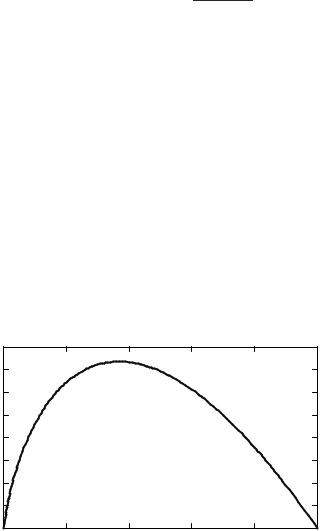
Proof: Consider the function f (t) = −t log t shown in Figure 17.1. It can be veriﬁed by differentiation that the function f (·) is concave. Also, f (0) = f (1) = 0. Hence the function is positive between 0 and 1. Consider the chord of the function from t to t + ν (where ν ≤ 12 ). The maximum absolute slope of the chord is at either end (when t = 0 or 1 − ν). Hence for 0 ≤ t ≤ 1 − ν, we have

|f (t) − f (t + ν)| ≤ max{f (ν), f (1 − ν)} = −ν log ν.

(17.27)

Let r(x) = |p(x) − q(x)|. Then

−

H (q)

| =

(

−

p(x) log p(x)

(17.28)

H (p)

q(x) log q(x))

≤ |(−p(x) log p(x) + q(x) log q(x))|

(17.29)

x X
0.4		f(t ) = −t In t
0.4
0.35
0.3
0.25
Int
0.2
−t
0.15
0.1
0.05
0	0.2	0.4	0.6	0.8	1
0	0.2	0.4	0.6	0.8	1
			t
	FIGURE 17.1. Function f (t) = −t ln t.

<<< < Предыдущая 54 55 56 57 58 59 60 61 62 63 64 65 66 67 6869 / 7869 70 71 72 73 74 75 76 77 78 > Следующая >>>

Соседние файлы в папке Теория информации

#
09.08.201310.58 Mб239Cover T.M., Thomas J.A. Elements of Information Theory. 2006., 748p.pdf
#
09.08.20131.32 Mб32Gray R.M. Entropy and information theory. 1990., 284p.pdf