

- •Block Reference
- •Commonly Used
- •Continuous
- •Discontinuities
- •Discrete
- •Logic and Bit Operations
- •Lookup Tables
- •Math Operations
- •Model Verification
- •Model-Wide Utilities
- •Ports & Subsystems
- •Signal Attributes
- •Signal Routing
- •Sinks
- •Sources
- •User-Defined Functions
- •Additional Math & Discrete
- •Additional Discrete
- •Additional Math: Increment — Decrement
- •Run on Target Hardware
- •Target for Use with Arduino Hardware
- •Target for Use with BeagleBoard Hardware
- •Target for Use with LEGO MINDSTORMS NXT Hardware
- •Blocks — Alphabetical List
- •Command-Line Information
- •Command-Line Information
- •Command-Line Information
- •Command-Line Information
- •Command-Line Information
- •Command-Line Information
- •Command-Line Information
- •Command-Line Information
- •Command-Line Information
- •Command-Line Information
- •Command-Line Information
- •Command-Line Information
- •Command-Line Information
- •Command-Line Information
- •Command-Line Information
- •Command-Line Information
- •Settings Pane
- •Measurements Pane
- •Signal Statistics Measurements
- •Settings Pane
- •Transitions Pane
- •Overshoots/Undershoots
- •Cycles
- •Settings Pane
- •Peaks Pane
- •Command-Line Information
- •Command-Line Information
- •Command-Line Information
- •Command-Line Information
- •Command-Line Information
- •Command-Line Information
- •Command-Line Information
- •Command-Line Information
- •Command-Line Information
- •Function Reference
- •Model Construction
- •Simulation
- •Linearization and Trimming
- •Data Type
- •Examples
- •Main Toolbar
- •Command-Line Alternative
- •Command-Line Alternative
- •Command-Line Alternative
- •Command-Line Alternative
- •Command-Line Alternative
- •Command-Line Alternative
- •Mask Icon Drawing Commands
- •Simulink Classes
- •Model Parameters
- •About Model Parameters
- •Examples of Setting Model Parameters
- •Common Block Parameters
- •About Common Block Parameters
- •Examples of Setting Block Parameters
- •Block-Specific Parameters
- •Mask Parameters
- •About Mask Parameters
- •Notes on Mask Parameter Storage
- •Simulink Identifier
- •Simulink Identifier
- •Model Advisor Checks
- •Simulink Checks
- •Simulink Check Overview
- •See Also
- •Identify unconnected lines, input ports, and output ports
- •Description
- •Results and Recommended Actions
- •Capabilities and Limitations
- •Tips
- •See Also
- •Check root model Inport block specifications
- •Description
- •Results and Recommended Actions
- •See Also
- •Check optimization settings
- •Description
- •Results and Recommended Actions
- •Tips
- •See Also
- •Description
- •Results and Recommended Actions
- •See Also
- •Check for implicit signal resolution
- •Description
- •Results and Recommended Actions
- •See Also
- •Check for optimal bus virtuality
- •Description
- •Results and Recommended Actions
- •Capabilities and Limitations
- •See Also
- •Description
- •Results and Recommended Actions
- •Capabilities and Limitations
- •See Also
- •Identify disabled library links
- •Description
- •Results and Recommended Actions
- •Capabilities and Limitations
- •Tips
- •See Also
- •Identify parameterized library links
- •Description
- •Results and Recommended Actions
- •Capabilities and Limitations
- •Tips
- •See Also
- •Identify unresolved library links
- •Description
- •Results and Recommended Actions
- •Capabilities and Limitations
- •See Also
- •Results and Recommended Actions
- •Capabilities and Limitations
- •See Also
- •Results and Recommended Actions
- •Capabilities and Limitations
- •See Also
- •Check usage of function-call connections
- •Description
- •Results and Recommended Actions
- •See Also
- •Check signal logging save format
- •Description
- •Results and Recommended Actions
- •See Also
- •Description
- •Results and Recommended Actions
- •See Also
- •Description
- •Results and Recommended Actions
- •Tips
- •See Also
- •Check data store block sample times for modeling errors
- •Description
- •Results and Recommended Actions
- •See Also
- •Check for potential ordering issues involving data store access
- •Description
- •Results and Recommended Actions
- •Tips
- •See Also
- •Check for partial structure parameter usage with bus signals
- •Description
- •Results and Recommended Actions
- •Tips
- •See Also
- •Check for calls to slDataTypeAndScale
- •Description
- •Results and Recommended Actions
- •Tips
- •See Also
- •Check for proper bus usage
- •Description
- •Results and Recommended Actions
- •Action Results
- •Tips
- •See Also
- •Description
- •Results and Recommended Actions
- •See Also
- •Description
- •Results and Recommended Actions
- •See Also
- •Check for proper Merge block usage
- •Description
- •Input Parameters
- •Results and Recommended Actions
- •See Also
- •Description
- •Results and Recommended Actions
- •Action Results
- •See Also
- •Check for non-continuous signals driving derivative ports
- •Description
- •Results and Recommended Actions
- •See Also
- •Runtime diagnostics for S-functions
- •Description
- •Results and Recommended Actions
- •See Also
- •Check file for foreign characters
- •Description
- •Results and Recommended Actions
- •Tips
- •See Also
- •Check model for known block upgrade issues
- •Description
- •Results and Recommended Actions
- •Action Results
- •See Also
- •Description
- •Results and Recommended Actions
- •Action Results
- •See Also
- •Check that the model is saved in SLX format
- •Description
- •Results and Recommended Actions
- •Tips
- •See Also
- •Check Model History properties
- •Description
- •Results and Recommended Actions
- •See Also
- •Analyze model hierarchy for upgrade issues
- •Description
- •Results and Recommended Actions
- •Tips
- •See Also
- •Description
- •Results and Recommended Actions
- •See Also
- •Simulink Performance Advisor Checks
- •Simulink Performance Advisor Check Overview
- •See Also
- •Baseline
- •See Also
- •Check Preupdate Items
- •See Also
- •Checks that need Update Diagram
- •See Also
- •Checks that require simulation to run
- •See Also
- •Check Accelerator Settings
- •See Also
- •Create Baseline
- •See Also
- •Identify resource intensive diagnostic settings
- •See Also
- •Check optimization settings
- •See Also
- •Identify inefficient lookup table blocks
- •See Also
- •Identify Interpreted MATLAB Function blocks
- •See Also
- •Check MATLAB Function block debug settings
- •See Also
- •Check Stateflow block debug settings
- •See Also
- •Identify simulation target settings
- •See Also
- •Check model reference rebuild setting
- •See Also
- •Check Model Reference parallel build
- •See Also
- •Check solver type selection
- •See Also
- •Select normal or accelerator simulation mode
- •See Also
- •Simulink Limits
- •Maximum Size Limits of Simulink Models
- •Index
- •Filter Structures and Filter Coefficients
- •Valid Initial States
- •Number of Delay Elements (Filter States)
- •Frame-Based Processing
- •Sample-Based Processing
- •Valid Initial States
- •Frame-Based Processing
- •Sample-Based Processing
- •Model Parameters in Alphabetical Order
- •Common Block Parameters
- •Continuous Library Block Parameters
- •Discontinuities Library Block Parameters
- •Discrete Library Block Parameters
- •Logic and Bit Operations Library Block Parameters
- •Lookup Tables Block Parameters
- •Math Operations Library Block Parameters
- •Model Verification Library Block Parameters
- •Model-Wide Utilities Library Block Parameters
- •Ports & Subsystems Library Block Parameters
- •Signal Attributes Library Block Parameters
- •Signal Routing Library Block Parameters
- •Sinks Library Block Parameters
- •Sources Library Block Parameters
- •User-Defined Functions Library Block Parameters
- •Additional Discrete Block Library Parameters
- •Additional Math: Increment - Decrement Block Parameters
- •Mask Parameters

5
Mask Icon Drawing
Commands
color |
Change drawing color of subsequent |
|
mask icon drawing commands |
disp |
Display text on masked subsystem |
|
icon |
dpoly |
Display transfer function on masked |
|
subsystem icon |
droots |
Display transfer function on masked |
|
subsystem icon |
fprintf |
Display variable text centered on |
|
masked subsystem icon |
image |
Display RGB image on masked |
|
subsystem icon |
patch |
Draw color patch of specified shape |
|
on masked subsystem icon |
plot |
Draw graph connecting series of |
|
points on masked subsystem icon |
port_label |
Draw port label on masked |
|
subsystem icon |
text |
Display text at specific location on |
|
masked subsystem icon |
color
Purpose
Syntax
Description
Examples
Change drawing color of subsequent mask icon drawing commands
color(colorstr)
color(colorstr) sets the drawing color of all subsequent mask drawing commands to the color specified by the string colorstr.
colorstr must be one of the following supported color strings.
blue green red cyan magenta yellow black
Entering any other string or specifying the color using RGB values results in a warning at the MATLAB command prompt; Simulink ignores the color change. The specified drawing color does not influence the color used by the patch or image drawing commands.
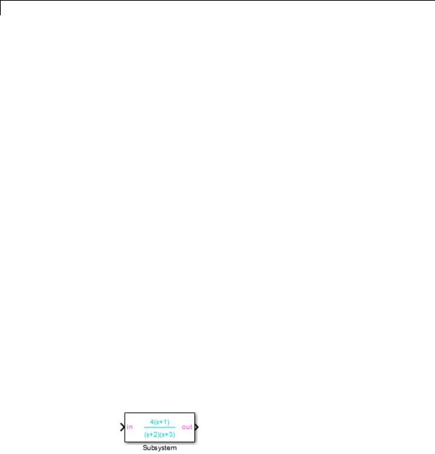
The following commands
color('cyan'); droots([-1], [-2 -3], 4) color('magenta') port_label('input',1,'in')
port_label('output',1,'out')
draw the following mask icon.
5-2

color
See Also droots | port_label
5-3
disp
Purpose |
Display text on masked subsystem icon |
Syntax |
disp(text) |
|
disp(text, 'texmode', 'on') |
Description |
disp(text) displays text centered on the block icon. text is any |
|
MATLAB expression that evaluates to a string. |
|
disp(text, 'texmode', 'on') allows you to use TeX formatting |
|
commands in text. The TeX formatting commands in turn allow you |
|
to include symbols and Greek letters in icon text. See “Mathematical |
|
Symbols, Greek Letters, and TeX Characters” in the MATLAB |
|
documentation for information on the TeX formatting commands |
|
supported by Simulink software. |
Examples |
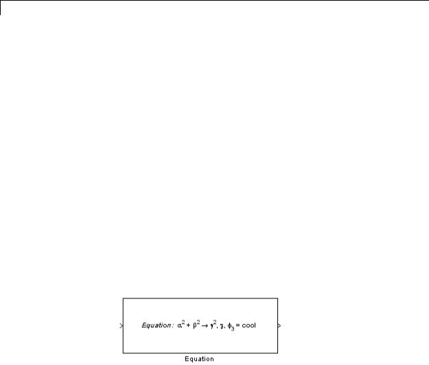
The following command |
|
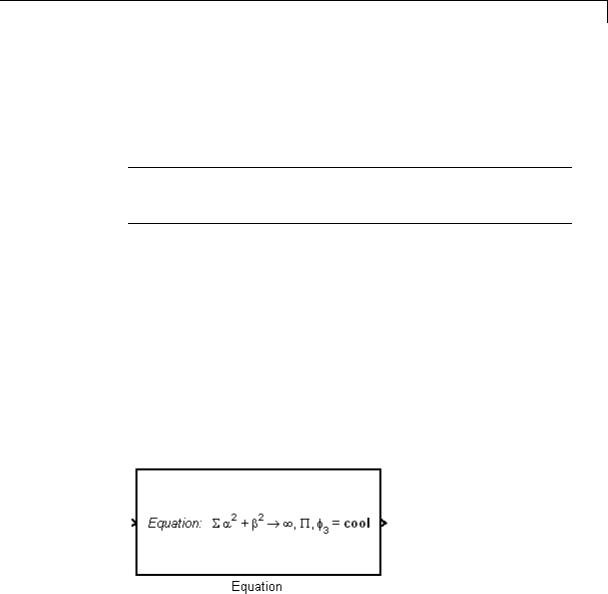
disp('{\itEquation:} \alpha^2 + \beta^2 \rightarrow \gamma^2, |
|
\chi, \phi_3 = {\bfcool}', 'texmode','on') |
|
draws the equation that appears on this masked block icon. |
See Also fprintf | port_label | text
5-4
dpoly
Purpose
Syntax
Description
Display transfer function on masked subsystem icon
dpoly(num, den)
dpoly(num, den, 'character')
dpoly(num, den) displays the transfer function whose numerator is num and denominator is den.
dpoly(num, den, 'character') specifies the name of the transfer function independent variable. The default is s.
When Simulink draws the block icon, the initialization commands execute and the resulting equation appears on the block icon, as in the following examples:
•To display a continuous transfer function in descending powers of s, enter
dpoly(num, den)
For example, for num = [0 0 1]; and den = [1 2 1] the icon looks like:
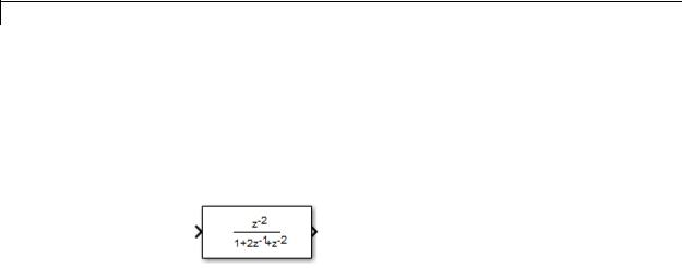
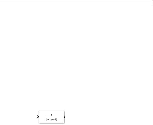
•To display a discrete transfer function in descending powers of z, enter
dpoly(num, den, 'z')
For example, for num = [0 0 1]; and den = [1 2 1]; the icon looks like:
5-5
dpoly
•To display a discrete transfer function in ascending powers of 1/z, enter
dpoly(num, den, 'z-')
For example, for num and den as defined previously, the icon looks like:
|
If the parameters are not defined or have no values when you create the |
|
icon, Simulink software displays three question marks (? ? ?) in the |
|
icon. When you define parameter values in the Mask Settings dialog |
|
box, Simulink software evaluates the transfer function and displays |
|
the resulting equation in the icon. |
See Also |
disp | port_label | text | droots |
5-6
droots
Purpose
Syntax
Description
See Also
Display transfer function on masked subsystem icon
droots(zero, pole, gain) droots(zero, pole, gain,'z') droots(zero, pole, gain,'z-')
droots(zero, pole, gain) displays the transfer function whose zero is zero, pole is pole, and gain is gain.
droots(zero, pole, gain,'z') and droots(zero, pole, gain,'z-') expresses the transfer function in terms of z or 1/z.
When Simulink draws the block icon, the initialization commands execute and the resulting equation appears on the block icon, as in the following examples:
•To display a zero-pole gain transfer function, enter droots(z, p, k)
For example, the preceding command creates this icon for these values:
z = []; p = [-1 -1]; k = 1;
If the parameters are not defined or have no values when you create the icon, Simulink software displays three question marks (? ? ?) in the icon. When you define parameter values in the Mask Settings dialog box, Simulink software evaluates the transfer function and displays the resulting equation in the icon.
disp | port_label | text | dpoly
5-7

fprintf
Purpose
Syntax
Description
Display variable text centered on masked subsystem icon
fprintf(text) fprintf(format, var)
The fprintf command displays formatted text centered on the icon and can display format along with the contents of var.
Note While this fprintf function is identical in name to its corresponding MATLAB function, it provides only the functionality described on this page.
Examples
See Also
The command
fprintf('Hello');
displays the string 'Hello' on the icon. The command
fprintf('Juhi = %d',17);
uses the decimal notation format (%d) to display the variable 17.
disp | port_label | text
5-8

image
Purpose
Syntax
Description
Display RGB image on masked subsystem icon
image(a)
image(a, position)
image(a, position, rotation)
image(a) displays the image a, where a is an m-by-n-by-3 array of RGB values. If necessary, use the MATLAB commands imread and ind2rgb to read and convert bitmap files (such as GIF) to the necessary matrix format.
image(a, position) creates the image at the specified position as follows.
|
Position |
Description |
|
|
[x, y, w, h] |
Position (x, y) and size (w, h) of the image |
|
|
|
where the position is relative to the lower-left |
|
|
|
corner of the mask. The image scales to fit the |
|
|
|
specified size. |
|
|
'center' |
Center of the mask |
|
|
|
|
|
|
'top-left' |
Top left corner of the mask, unscaled |
|
|
|
|
|
|
'bottom-left' |
Bottom left corner of the mask, unscaled |
|
|
|
|
|
|
'top-right' |
Top right corner of the mask, unscaled |
|
|
|
|
|
|
'bottom-right' |
Bottom right corner of the mask, unscaled |
|
|
|
|
|
image(a, position, rotation) allows you to specify whether the image rotates ('on') or remains stationary ('off') as the icon rotates. The default is 'off'.
5-9

image
Examples
See Also
The command
image(imread('icon.jpg'))
reads the icon image from a JPEG file named icon.jpg in the MATLAB path.
The following commands read and convert a GIF file, label.gif, to the appropriate matrix format. You can type these commands in the Initialization pane of the Mask Editor.
[data, map]=imread('label.gif'); pic=ind2rgb(data,map);
Then type the command
image(pic)
in the Icon pane of the Mask Editor to read the converted label image.
patch | plot
5-10
patch
Purpose
Syntax
Description
Examples
See Also
Draw color patch of specified shape on masked subsystem icon
patch(x, y)
patch(x, y, [r g b])
patch(x, y) creates a solid patch having the shape specified by the coordinate vectors x and y. The patch’s color is the current foreground color.
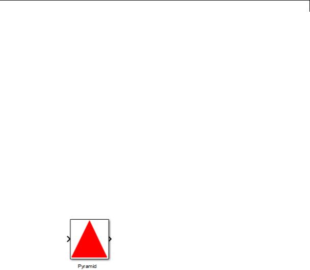
patch(x, y, [r g b]) creates a solid patch of the color specified by the vector [r g b], where r is the red component, g the green, and b the blue. For example,
patch([0 .5 1], [0 1 0], [1 0 0])
creates a red triangle on the mask’s icon.
The command
patch([0 .5 1], [0 1 0], [1 0 0])
creates a red triangle on the mask’s icon.
image | plot
5-11

plot
Purpose
Syntax
Description
Examples
Draw graph connecting series of points on masked subsystem icon
plot(Y) plot(X1,Y1,X2,Y2,...)
plot(Y) plots, for a vector Y, each element against its index. If Y is a matrix, it plots each column of the matrix as though it were a vector.
plot(X1,Y1,X2,Y2,...) plots the vectors Y1 against X1, Y2 against X2, and so on. Vector pairs must be the same length and the list must consist of an even number of vectors.
Plot commands can include NaN and inf values. When Simulink software encounters NaNs or infs, it stops drawing, and then begins redrawing at the next numbers that are not NaN or inf. The
appearance of the plot on the icon depends on the value of the Drawing coordinates parameter.
Simulink software displays three question marks (? ? ?) in the block icon and issues warnings in these situations:
•When you have not defined values for the parameters used in the drawing commands (for example, when you first create the mask, but have not yet entered values in the Mask Settings dialog box)
•When you enter a masked block parameter or drawing command incorrectly
The command
plot([0 1 5], [0 0 4])
generates the plot that appears on the icon for the Ramp block, in the Sources library.
5-12

plot
See Also |
image |
5-13

port_label
Purpose
Syntax
Description
Draw port label on masked subsystem icon
port_label('port_type', port_number, 'label') port_label('port_type', port_number, 'label', 'texmode', 'on')
port_label('port_type', port_number, 'label') draws a label on a port. Valid values for port_type include the following.
|
Value |
Description |
|
|
input |
Simulink input port |
|
|
output |
Simulink output port |
|
|
lconn |
Physical Modeling connection port on the left side |
|
|
|
of a masked subsystem |
|
|
rconn |
Physical Modeling connection port on the right |
|
|
|
side of a masked subsystem |
|
The input argument port_number is an integer, and label is a string specifying the port’s label.
Note Physical Modeling port labels are assigned based on the nominal port location. If the masked subsystem has been rotated or flipped, for example, a port labeled using 'lconn' as the port_type may not appear on the left side of the block.
port_label('port_type', port_number, 'label', 'texmode', 'on') lets you use TeX formatting commands in label. The TeX formatting commands allow you to include symbols and Greek letters in the port label. See “Mathematical Symbols, Greek Letters, and TeX Characters” in the MATLAB documentation for information on the TeX formatting commands that the Simulink software supports.
5-14
port_label
Examples
See Also
The command
port_label('input', 1, 'a')
defines a as the label of input port 1. The commands
disp('Card\nSwapper'); port_label('input',1,'\spadesuit','texmode','on'); port_label('output',1,'\heartsuit','texmode','on');
draw playing card symbols as the labels of the ports on a masked subsystem.
disp | fprintf | text
5-15

text
Purpose
Syntax
Description
Display text at specific location on masked subsystem icon
text(x, y, 'text')
text(x, y, 'text', 'horizontalAlignment', 'halign', 'verticalAlignment', 'valign')
text(x, y, 'text', 'texmode', 'on')
The text command places a character string at a location specified by the point (x,y). The units depend on the Drawing coordinates parameter.
text(x,y, text, 'texmode', 'on') allows you to use TeX formatting commands in text. The TeX formatting commands in turn allow you to include symbols and Greek letters in icon text. See “Mathematical Symbols, Greek Letters, and TeX Characters” in the MATLAB documentation for information on the TeX formatting commands supported by Simulink software.
You can optionally specify the horizontal and/or vertical alignment of the text relative to the point (x, y) in the text command.
The text command offers the following horizontal alignment options.
|
Option |
Aligns |
|
|
'left' |
The left end of the text at the specified point |
|
|
'right' |
The right end of the text at the specified point |
|
|
'center' |
The center of the text at the specified point |
|
|
|
|
|
The text command offers the following vertical alignment options.
|
Option |
Aligns |
|
|
'base' |
The baseline of the text at the specified point |
|
|
'bottom' |
The bottom line of the text at the specified point |
|
|
'middle' |
The midline of the text at the specified point |
|
|
|
|
|
5-16
text
Examples
|
Option |
Aligns |
|
|
'cap' |
The capitals line of the text at the specified point |
|
|
'top' |
The top of the text at the specified point |
|
|
|
|
|
Note While this text function is identical in name to its corresponding MATLAB function, it provides only the functionality described on this page.
The command
text(0.5, 0.5, 'foobar', 'horizontalAlignment', 'center')
centers foobar in the icon. The command
text(.05,.5,'{\itEquation:} \Sigma \alpha^2 + \beta^2 \rightarrow \infty, \Pi, \phi_3 = {\bfcool}', 'hor','left','texmode','on')
draws a left-aligned equation on the icon.
See Also disp | fprintf | port_label
5-17

text
5-18

6
Simulink Debugger
Commands
animate |
Enable or disable animation mode |
ashow |
Show algebraic loop |
atrace |
Set algebraic loop trace level |
bafter |
Insert breakpoint after specified |
|
method |
break |
Insert breakpoint before specified |
|
method |
bshow |
Show specified block |
clear |
Clear breakpoints from model |
continue |
Continue simulation |
disp |
Display block’s I/O when simulation |
|
stops |
ebreak |
Enable (or disable) breakpoint on |
|
solver errors |
elist |
List simulation methods in order |
|
in which they are executed during |
|
simulation |
emode |
Toggle model execution between |
|
accelerated and normal mode |
etrace |
Enable or disable method tracing |
help |
Display help for debugger commands |

6 Simulink® Debugger Commands
nanbreak |
Set or clear nonfinite value break |
|
mode |
next |
Advance simulation to start of next |
|
method at current level in model’s |
|
execution list |
probe |
I/O and state data for blocks |
quit |
Stop simulation debugger |
rbreak |
Break simulation before solver reset |
run |
Run simulation to completion |
slist |
Sorted list of model blocks |
states |
Current state values |
status |
Debugging options in effect |
step |
Advance simulation by one or more |
|
methods |
stimes |
Model sample times |
stop |
Stop simulation |
strace |
Set solver trace level |
systems |
List nonvirtual systems of model |
tbreak |
Set or clear time breakpoint |
trace |
Display block’s I/O each time block |
|
executes |
undisp |
Remove block from debugger’s list of |
|
display points |
untrace |
Remove block from debugger’s list of |
|
trace points |
where |
Display current location of |
|
simulation in simulation loop |
xbreak |
Break when debugger encounters |
|
step-size-limiting state |
6-2

zcbreak |
Toggle breaking at nonsampled |
|
zero-crossing events |
zclist |
List blocks containing nonsampled |
|
zero crossings |
6-3

animate
Purpose
Syntax
Short
Form
Arguments
Description
See Also
Enable or disable animation mode
animate [delay | stop]
ani
delay Length in seconds between method calls (1 second by default).
stop Disable animation mode.
animate without any arguments enables animation mode. animate delay enables animation mode and specifies delay as the time delay in seconds between method calls. animate stop disables animation mode.
continue
6-4

ashow
Purpose
Syntax
Short
Form
Arguments
Description
See Also
Show algebraic loop
ashow <gcb | s:b | s#n | clear>
as
gcb Current block.
s:b The block whose system index is s and block index is b. s#n The algebraic loop numbered n in system s.
clear Switch that clears loop coloring.
ashow without any arguments lists all of a model’s algebraic loops in the MATLAB Command Window. ashow gcb or ashow s:b highlights the algebraic loop that contains the specified block. ashow s#n highlights the nth algebraic loop in system s. The ashow clear command removes algebraic loop highlights from the model diagram.
atrace | slist
6-5

atrace
Purpose
Syntax
Short
Form
Arguments
Description
See Also
Set algebraic loop trace level
atrace level
at
level Trace level (0 = none, 4 = everything).
The atrace command sets the algebraic loop trace level for a simulation.
|
Command |
|
Displays for Each Algebraic Loop |
|
|
atrace 0 |
|
No information |
|
|
atrace 1 |
|
The loop variable solution, the number of iterations |
|
|
|
|
required to solve the loop, and the estimated |
|
|
|
|
solution error |
|
|
atrace 2 |
|
Same as level 1 |
|
|
atrace 3 |
|
Level 2 plus Jacobian matrix used to solve loop |
|
|
atrace 4 |
|
Level 3 plus intermediate solutions of the loop |
|
|
|
|
variable |
|
|
states | systems |
|
|
|
6-6
bafter
Purpose |
Insert breakpoint after specified method |
Syntax |
bafter |
|
bafter m:mid |
|
bafter <sysIdx:blkIdx | gcb> [mth] [tid:TID] |
|
bafter <s:sysIdx | gcs> [mth] [tid:TID] |
|
bafter model [mth] [tid:TID] |
Short
Form
Arguments
Description
ba
mid Method ID
|
Block ID |
sysIdx:blkIdx |
|
gcb |
Currently selected block |
sysIdx |
System ID |
gcs |
Currently selected system |
model |
Currently selected model |
mth |
A method name, e.g., Outputs.Major |
TID |
Task ID |
bafter inserts a breakpoint after the current method.
bafter m:mid inserts a breakpoint after the method specified by mid (see “Method ID”).
bafter sysIdx:blkIdx inserts a breakpoint after each invocation of the method of the block specified by sysIdx:blkIdx (see “Block ID”) in major time steps. bafter gcb inserts a breakpoint after each
invocation of a method of the currently selected block (see gcb) in major times steps.
6-7

bafter
|
bafter s:sysIdx inserts a breakpoint after each method of the root |
|
system or nonvirtual subsystem specified by the system ID: sysIdx. |
|
|
|
Note The systems command displays the system IDs for all nonvirtual |
|
systems in the currently selected model. |
|
|
|
bafter gcs inserts a breakpoint after each method of the currently |
|
selected nonvirtual system. |
|
bafter model inserts a breakpoint after each method of the currently |
|
selected model. |
|
The optional mth parameter allow you to set a breakpoint after a |
|
particular block, system, or model method and task. For example, |
|
bafter gcb Outputs sets a breakpoint after the Outputs method of |
|
the currently selected block. |
|
The optional TID parameter allows you to set a breakpoint after |
|
invocation of a method by a particular task. For example, suppose that |
|
the currently selected nonvirtual subsystem operates on task 2 and 3. |
|
Then bafter gcs Outputs tid:2 sets a breakpoint after the invocation |
|
of the subsystem’s Outputs method that occurs when task 2 is active. |
See Also |
break | ebreak | tbreak | xbreak | nanbreak | zcbreak | rbreak | |
|
clear | where | slist | systems |
6-8

break
Purpose |
Insert breakpoint before specified method |
Syntax |
break |
|
break m:mid |
|
break <sysIdx:blkIdx | gcb> [mth] [tid:TID] |
|
break <s:sysIdx | gcs> [mth] [tid:TID] |
|
break model [mth] [tid:TID] |
Short
Form
Arguments
Description
b
mid Method ID
|
Block ID |
sysIdx:blkIdx |
|
gcb |
Currently selected block |
sysIdx |
System ID |
gcs |
Currently selected system |
model |
Currently selected model |
mth |
A method name, e.g., Outputs.Major |
TID |
task ID |
break inserts a breakpoint before the current method.
break m:mid inserts a breakpoint before the method specified by mid (see “Method ID”).
break sysIdx:blkIdx inserts a breakpoint before each invocation of the method of the block specified by sysIdx:blkIdx (see “Block ID”) in major time steps. break gcb inserts a breakpoint before each invocation of a method of the currently selected block (see gcb) in major times steps.
break s:sysIdx inserts a breakpoint at each method of the root system or nonvirtual subsystem specified by the system ID: sysIdx.
6-9

break
|
Note The systems command displays the system IDs for all nonvirtual |
|
systems in the currently selected model. |
|
|
|
break gcs inserts a breakpoint at each method of the currently selected |
|
nonvirtual system. |
|
break model inserts a breakpoint at each method of the currently |
|
selected model. |
|
The optional mth parameter allow you to set a breakpoint at a particular |
|
block, system, or model method. For example, break gcb Outputs sets |
|
a breakpoint at the Outputs method of the currently selected block. |
|
The optional TID parameter allows you to set a breakpoint at the |
|
invocation of a method by a particular task. For example, suppose that |
|
the currently selected nonvirtual subsystem operates on task 2 and 3. |
|
Then break gcs Outputs tid:2 sets a breakpoint at the invocation of |
|
the subsystem’s Outputs method that occurs when task 2 is active. |
See Also |
bafter | clear | ebreak | nanbreak | rbreak | systems | tbreak | |
|
where | xbreak | zcbreak | slist |
6-10

bshow
Purpose
Syntax
Short
Form
Arguments
Description
See Also
Show specified block
bshow s:b
bs
s:b The block whose system index is s and block index is b.
The bshow command opens the model window containing the specified block and selects the block.
slist
6-11

clear
Purpose |
Clear breakpoints from model |
Syntax |
clear |
|
clear m:mid |
|
clear id |
|
clear <sysIdx:blkIdx | gcb> |
Arguments
Description
See Also
Short Form cl
mid |
Method ID |
id |
Breakpoint ID |
sysIdx:blkIdxBlock ID
gcb Currently selected block
clear clears a breakpoint from the current method.
clear m:mid clears a breakpoint from the method specified by mid. clear id clears the breakpoint specified by the breakpoint ID id.
clear sysIdx:blkIdx clears any breakpoints set on the methods of the block specified by sysIdx:blkIdx.
clear gcb clears any breakpoints set on the methods of the currently selected block.
break | bafter | slist
6-12

continue
Purpose |
Continue simulation |
Syntax |
continue |
Short |
c |
Form |
|
Description |
The continue command continues the simulation from the current |
|
breakpoint. If animation mode is not enabled, the simulation continues |
|
until it reaches another breakpoint or its final time step. If animation |
|
mode is enabled, the simulation continues in animation mode to the |
|
first method of the next major time step, ignoring breakpoints. |
See Also |
run | stop | quit | animate |
6-13

disp
Purpose |
Display block’s I/O when simulation stops |
Syntax |
disp |
|
disp gcb |
|
disp s:b |
Short Form d
Arguments
Description
See Also
s:b The block whose system index is s and block index is b. gcb Current block.
The disp command registers a block as a display point. The debugger displays the inputs and outputs of all display points in the MATLAB Command Window whenever the simulation halts. Invoking disp without arguments shows a list of display points. Use undisp to unregister a block.
undisp | slist | probe | trace
6-14

ebreak
Purpose |
Enable (or disable) breakpoint on solver errors |
Syntax |
ebreak |
Short |
eb |
Form |
|
Description |
This command causes the simulation to stop if the solver detects |
|
a recoverable error in the model. If you do not set or disable this |
|
breakpoint, the solver recovers from the error and proceeds with the |
|
simulation without notifying you. |
See Also |
break | bafter | tbreak | xbreak | nanbreak | zcbreak | rbreak | |
|
clear | where | slist | systems |
6-15
elist
Purpose |
List simulation methods in order in which they are executed during |
|
|
simulation |
|
Syntax |
elist m:mid [tid:TID] |
|
|
elist |
<gcs | s:sysIdx> [mth] [tid:TID] |
|
elist |
<gcb | sysIdx:blkIdx> [mth] [tid:TID] |
Short Form el
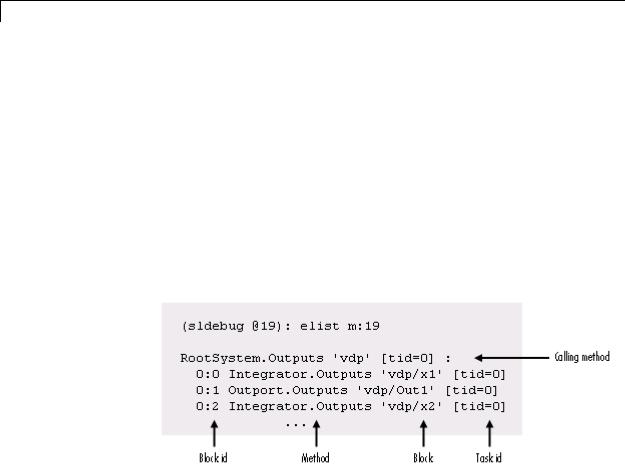
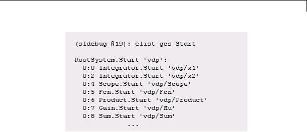
Description elist m:mid lists the methods invoked by the system or nonvirtual subsystem method corresponding to the method id mid (see the where command for information on method IDs), e.g.,
The method list specifies the calling method followed by the methods that it calls in the order in which they are invoked. The entry for the calling method includes
•The name of the method
The name of the method is prefixed by the type of system that defines the method, e.g., RootSystem.
•The name of the model or subsystem instance on which the method is invoked
•The ID of the task that invokes the method
6-16
elist
The entry for each called method includes
•The ID (sysIdx:blkIdx) of the block instance on which the method is invoked
The block ID is prefixed by a number specifying the system that contains the block (the sysIdx). This allows Simulink software to assign the same block ID to blocks residing in different subsystems.
•The name of the method
The method name is prefixed with the type of block that defines the method, e.g., Integrator.
•The name of the block instance on which the method is invoked
•The task that invokes the method
The optional task ID parameter (tid:TID) allows you to restrict the displayed lists to methods invoked for a specified task. You can specify this option only for system or atomic subsystem methods that invoke Outputs or Update methods.
elist <gcs | s:sysIdx> lists the methods executed for the currently selected system (specified by the gcs command) or the system or nonvirtual subsystem specified by the system ID sysIdx, e.g.,
6-17
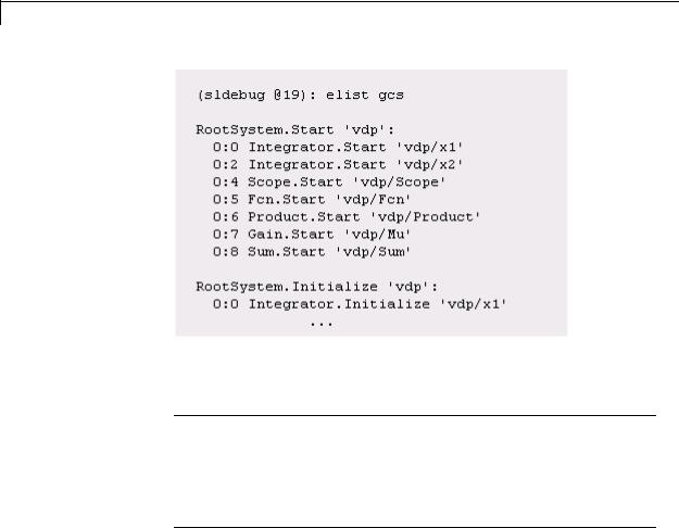
elist
The system ID of a model’s root system is 0. You can use the debugger’s systems command to determine the system IDs of a model’s subsystems.
Note The elist and where commands use block IDs to identify subsystems in their output. The block ID for a subsystem is not the same as the system ID displayed by the systems command. Use the elist sysIdx:blkIdx form of the elist command to display the methods of a subsystem whose block ID appears in the output of a previous invocation of the elist or where command.
elist <gcs | s:sysIdx> mth lists methods of type mth to be executed for the system specified by the gcs command or the system ID sysIdx, e.g.,
6-18
elist
Use elist gcb to list the methods invoked by the nonvirtual subsystem currently selected in the model.
See Also where | slist | systems
6-19

emode
Purpose |
Toggle model execution between accelerated and normal mode |
Syntax |
emode |
Short |
em |
Form |
|
Description |
Toggles the simulation between accelerated and normal mode when |
|
using the Accelerator mode in Simulink software. For more information, |
|
see “Run Accelerator Mode with the Simulink Debugger”. |
6-20

etrace
Purpose |
Enable or disable method tracing |
Syntax |
etrace level level-number |
|
Short Form |
|
et |
Description
See Also
This command enables or disables method tracing, depending on the value of level:
Level Description
0Turn tracing off.
1Trace model methods.
2Trace model and system methods.
3Trace model, system, and block methods.
When method tracing is on, the debugger prints a message at the command line every time a method of the specified level is entered or exited. The message specifies the current simulation time, whether the simulation is entering or exiting the method, the method id and name, and the name of the model, system, or block to which the method belongs.
elist | where | trace
6-21

help
Purpose |
Display help for debugger commands |
Syntax |
help |
Short |
? or h |
Form |
|
Description |
The help command displays a list of debugger commands in the |
|
command window. The list includes the syntax and a brief description |
|
of each command. |
6-22

nanbreak
Purpose
Syntax
Short
Form
Description
See Also
How To
Set or clear nonfinite value break mode
nanbreak
na
The nanbreak command causes the debugger to break whenever the simulation encounters a nonfinite (NaN or Inf) value. If nonfinite break mode is set, nanbreak clears it.
break | bafter | rbreak | tbreak | xbreak | zcbreak
• ebreak
6-23

next
Purpose |
Advance simulation to start of next method at current level in model’s |
|
execution list |
Syntax |
next |
Short |
n |
Form |
|
Description |
The next command advances the simulation to the start of the next |
|
method at the current level in the model’s method execution list. |
|
|
|
Note The next command has the same effect as the step over |
|
command. See step for more information. |
See Also |
|
step |
6-24

probe
Purpose
Syntax
Description
Examples
I/O and state data for blocks
probe probe s:b probe gcb
probe level level-type p
probe sets the Simulink debugger to interactive probe mode. In this mode, the debugger displays the I/O of a selected block. To exit
interactive probe mode, enter a debugger command or press the Enter key.
probe s:b displays the I/O of the block whose system index is s and block index is b.
probe gcb displays the I/O of the currently selected block.
probe level level-type sets the verbosity level for probe, trace, and dis. If level-type is io, the debugger displays block I/O. If level-type is all (default), the debugger displays all information for the current state of a block, including inputs and outputs, states, and zero crossings.
p is the short form of the command.
Display I/O for the currently selected block Out2 in the model vdp using the Simulink debugger.
1In the MATLAB Command Window, enter: sldebug 'vdp'
The MATLAB command prompt >> changes to the Simulink debugger prompt (sldebug @0): >>.
2Enter: probe gcb
6-25

probe
The MATLAB Command Window displays:
|
probe: |
Data of 0:3 Outport block 'vdp/Out2': |
|
U1 |
= [0] |
See Also |
disp | trace |
|
6-26
quit
Purpose |
Stop simulation debugger |
Syntax |
quit |
|
q |
Description |
quit stops the Simulink debugger and returns to the MATLAB |
|
command prompt. |
|
q is the short form of the command. |
Examples |
Start the Simulink debugger for the model vdp and then stop it. |
|
1 In the MATLAB Command Window, enter: |
|
sldebug 'vdp' |
|
The MATLAB command prompt >> changes to the Simulink |
|
debugger prompt (sldebug @0): >>. |
|
2 Enter: |
|
quit |
See Also |
stop |
6-27

rbreak
Purpose
Syntax
Description
Examples
See Also
Break simulation before solver reset
rbreak rb
rbreak enables (or disables) a solver reset breakpoint if the breakpoint is disabled (or enabled). The breakpoint causes the debugger to halt the simulation whenever an event requires a solver reset. The halt occurs before the solver resets.
rb is the short form of the command.
Start Simulink debugger for the model vdp and a set breakpoint before a solver reset.
1In the MATLAB Command Window, enter: sldebug 'vdp'
The MATLAB command prompt >> is replaced with the Simulink debugger prompt (sldebug @0): >>.
2Enter: rbreak
The MATLAB Command Window displays:
Break on solver reset request |
: enabled |
break | bafter | nanbreak | ebreak | tbreak | xbreak | zcbreak
6-28

run
Purpose |
Run simulation to completion |
Syntax |
run |
|
r |
Description |
run starts the simulation from the current breakpoint to its final time |
|
step. It ignores breakpoints and display points. |
|
r is the short form of the command |
Examples |
Continue the simulation for the model vdp using the Simulink debugger. |
|
1 In the MATLAB Command Window, enter: |
|
sldebug 'vdp' |
|
The MATLAB command prompt >> changes to the Simulink |
|
debugger prompt (sldebug @0): >>. |
|
2 Enter: |
|
run |
See Also |
continue | stop | quit |
6-29

slist
Purpose |
Sorted list of model blocks |
Syntax slist
sli
Description slist displays a list of blocks for the root system and each nonvirtual subsystem sorted according to data dependencies and other criteria.
For each system (root or nonvirtual), slist displays:
•Title line specifying the name of the system, the number of nonvirtual blocks that the system contains, and the number of blocks in the system that have direct feedthrough ports.
•Entry for each block in the order in which the blocks appear in the sorted list.
For each block entry, slist displays the block ID and the name and type of the block. The block ID consists of a system index and a block index separated by a colon (sysIdx:blkIdx).
•Block index is the position of the block in the sorted list.
•System index is the order in which the Simulink software generated the system sorted list. The system index has no special significance. It simply allows blocks that appear in the same position in different sorted lists to have unique identifiers.
Simulink software uses sorted lists to create block method execution lists (see elist) for root system and nonvirtual subsystem methods. In general, root system and nonvirtual subsystem methods invoke the block methods in the same order as the blocks appear in the sorted list.
Exceptions occur in the execution order of block methods. For example, execution lists for multicast models group together all blocks operating at the same rate and in the same task. Slower groups appear later than faster groups. The grouping of methods by task can result in a block method execution order that is different from the block sorted order. However, within groups, methods execute in the same order as the corresponding blocks appear in the sorted list.
6-30

slist
Examples
See Also
sli is the short form of the command.
Display a sorted list of the root system in the vdp model using the Simulink debugger.
1In the MATLAB Command Window, enter: sldebug 'vdp'
The MATLAB command prompt >> changes to the Simulink debugger prompt (sldebug @0): >>.
2Enter: slist
The MATLAB Command Window displays:
----Sorted list for 'vdp' [9 nonvirtual blocks, directFeed=0] 0:0 'vdp/x1' (Integrator)
0:1 'vdp/Out1' (Outport) 0:2 'vdp/x2' (Integrator) 0:3 'vdp/Out2' (Outport) 0:4 'vdp/Scope' (Scope) 0:5 'vdp/Fcn' (Fcn)
0:6 'vdp/Product' (Product) 0:7 'vdp/Mu' (Gain)
0:8 'vdp/Sum' (Sum)
systems | elist
6-31

states
Purpose
Syntax
Description
Examples
Current state values
states
states displays a list of the current states of the model. The list includes the index, current value, system:block:element ID, state vector name, and block name for each state.
Display information about the states for the vdp model.
1In the MATLAB Command Window, enter: sldebug 'vdp'
The MATLAB command prompt >> changes to the Simulink debugger prompt (sldebug @0): >>.
2Enter: states
The MATLAB Command Window displays:
Continuous States: |
|
|
|
|
|
Idx |
Value |
(system:block:element Name |
'BlockName |
||
0 |
0 |
(0:0:0 |
CSTATE |
'vdp/x1') |
|
1 |
0 |
(0:2:0 |
CSTATE |
'vdp/x2') |
|
6-32

status
Purpose
Syntax
Description
Examples
Debugging options in effect
status
status displays a list of the debugging options in effect.
Display status for the model vdp using the Simulink debugger.
1In the MATLAB Command Window, enter: sldebug 'vdp'
The MATLAB command prompt >> changes to the Simulink debugger prompt (sldebug @0): >>.
2Enter: status
The MATLAB Command Window displays:
%---------------------------------------------------------------- |
% |
Current simulation time |
: 0 (MajorTimeStep) |
Solver needs reset |
: no |
Solver derivatives cache needs reset |
: no |
Zero crossing signals cache needs reset |
: no |
Default command to execute on return/enter : "" |
|
Break at zero crossing events |
: disabled |
Break on solver error |
: disabled |
Break on failed integration step |
: disabled |
Time break point |
: disabled |
Break on non-finite (NaN,Inf) values |
: disabled |
Break on solver reset request |
: disabled |
Display level for disp, trace, probe |
: 1 (i/o, states) |
Solver trace level |
: 0 |
Algebraic loop tracing level |
: 0 |
Animation Mode |
: off |
Window reuse |
: not supported |
6-33

status
Execution Mode |
: Normal |
||
Display |
level for etrace |
: 0 (disabled) |
|
Break points |
: none |
installed |
|
Display |
points |
: none |
installed |
6-34

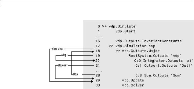
step
Purpose |
Advance simulation by one or more methods |
Syntax |
step |
|
step in |
|
step over |
|
step out |
|
step top |
|
step blockmth |
|
s |
Description |
step or step in advances the simulation to the next method in the |
|
current time step. |
|
step over advances the simulation over the next method. |
|
step out advances the simulation the end of the current simulation |
|
point hierarchy. |
|
step top advances the simulation to the first method executed in the |
|
next time step. |
|
step blockmth advances the simulation to the next method that |
|
operates on a block. |
|
s is the short form of the command. |
|
If step advances the simulation to the start of a block method, the |
|
debugger points at the block on which the method operates. |
|
. |
Examples |
The following diagram illustrates the effect of various forms of the step |
|
command for the model vdp. |
6-35
step
See Also next | where | elist
6-36
stimes
Purpose
Syntax
Description
Examples
Model sample times
stimes sti
stimes displays information about the model sample times, including the sample time period, offset, and task ID.
sti is the short form of the command.
Display sample times for the model vdp using the Simulink debugger.
1In the MATLAB Command Window, enter: sldebug 'vdp'
The MATLAB command prompt >> changes to the Simulink debugger prompt (sldebug @0): >>.
2Enter: stimes
The MATLAB Command Window displays:
--- Sample times |
for |
'vdp' [Number of sample times = |
1] |
|
1. [0 |
, 0 |
] |
tid=0 (continuous sample time) |
|
6-37

stop
Purpose |
Stop simulation |
Syntax |
stop |
Description |
stop stops the simulation of the model you are debugging. |
Examples |
Start and stop a simulation for the model vdp using the Simulink |
|
debugger. |
1Start a debugger session. In the MATLAB Command Window, enter: sldebug 'vdp'
The MATLAB command prompt >> changes to the Simulink debugger prompt (sldebug @0): >>.
2Start a simulation of the model. Enter: run
3Stop the simulation. Enter: stop
See Also continue | run | quit
6-38

strace
Purpose
Syntax
Description
Examples
Set solver trace level
strace level i
strace level causes the solver to display diagnostic information in the MATLAB Command Window, depending on the value of level. Values are 0 (no information) or 1 (maximum information about time steps, integration steps, zero crossings, and solver resets).
i is the short form of the command.
Display maximum information about a simulation for the model vdp using the Simulink debugger.
1In the MATLAB Command Window, enter: sldebug 'vdp'
The MATLAB command prompt >> changes to the Simulink debugger prompt (sldebug @0): >>.
2Get information about the notation . Enter: help time
The MATLAB Command Window displays:
Time is displayed as:
TM = <time while in MajorTimeStep> Tm = <time while in MinorTImeStep>
Ts = <time of successful integration step> Tf = <time of failed integration step>
Tr = <time of solver reset>
Tj = <time of Jacobian evaluation> (when using implicit solvers) Tz = <time at left post of interval bracketing zero crossing event
Step size is displayed as: H = <step size>
6-39

strace
Hs = <failed integration step size>
Hf = failed integration step size>
Hr = <step size at sovler reset>
Hz = <step size at zero crossing event>
Izc= <length of time interval bracketing zero crossing eent(s)>
3Set trace to display all information. Enter: strace 1
When diagnostic tracing is on, the debugger displays the sizes of major and minor time steps.
[TM = 13.21072088374186 ] Start of Major Time Step
[Tm = 13.21072088374186 ] Start of Minor Time Step
The debugger displays integration information. This information includes the time step of the integration method, step size of the integration method, outcome of the integration step, normalized error, and index of the state.
[Tm = 13.21072088374186 ] [H = 0.2751116230148764 ] Begin Integration Step
[Tf = 13.48583250675674 ] [Hf = 0.2751116230148764 ] Fail [Er = 1.0404e+000]
[Ix = 1]
[Tm = 13.21072088374186 ] [H = 0.2183536061326544 ] Retry
[Ts = 13.42907448987452 ] [Hs = 0.2183536061326539 ] Pass [Er = 2.8856e-001] [Ix = 1]
For zero crossings, the debugger displays information about the iterative search algorithm when the zero crossing occurred. This information includes the time step of the zero crossing, step size of the zero crossing detection algorithm, length of the time interval bracketing the zero crossing, and a flag denoting the rising or falling direction of the zero crossing.
[Tz = 3.615333333333301 ] Detected 1 Zero Crossing Event 0[F]
Begin iterative search to bracket zero crossing event [Tz = 3.621111157580072 ] [Hz = 0.005777824246771424 ] [Iz = 4.2222e-003] 0[F] [Tz = 3.621116982080098 ] [Hz = 0.005783648746797265 ] [Iz = 4.2164e-003] 0[F]
6-40

strace
[Tz = 3.621116987943544 ] [Hz = 0.005783654610242994 ] [Iz = 4.2163e-003] 0[F] [Tz = 3.621116987943544 ] [Hz = 0.005783654610242994 ] [Iz = 1.1804e-011] 0[F] [Tz = 3.621116987949452 ] [Hz = 0.005783654616151157 ] [Iz = 5.8962e-012] 0[F] [Tz = 3.621116987949452 ] [Hz = 0.005783654616151157 ] [Iz = 5.1514e-014] 0[F]
End iterative search to bracket zero crossing event
When a solver resets occur, the debugger displays the time at which the solver was reset.
|
[Tr = 6.246905153573676 |
] Process Solver Reset |
|
[Tr = 6.246905153573676 |
] Reset Zero Crossing Cache |
|
[Tr = 6.246905153573676 |
] Reset Derivative Cache |
See Also |
atrace | etrace | states | trace | zclist |
|
6-41

systems
Purpose
Syntax
Description
Examples
See Also
List nonvirtual systems of model
systems sys
systems displays the nonvirtual subsystems for a model in the MATLAB Command Window.
sys is the short form of the command.
Display the nonvirtual systems for the model sldemo_enginewc using the Simulink debugger.
1In the MATLAB Command Window, enter: sldebug 'sldemo_enginewc'
The MATLAB command prompt >> changes to the Simulink debugger prompt (sldebug @0): >>.
2Enter: systems
The MATLAB Command Window displays the nonvirtual subsystems.
0'sldemo_enginewc'
1'sldemo_enginewc/Compression'
2'sldemo_enginewc/Controller/TmpAtomicSubsysAtSwitchInport3'
3'sldemo_enginewc/Controller/TmpAtomicSubsysAtSwitchInport1'
4'sldemo_enginewc/Controller'
5'sldemo_enginewc/Throttle & Manifold/Throttle/TmpAtomicSubsysAtSw
6'sldemo_enginewc/valve timing/positive edge to dual edge conversi
slist
6-42

tbreak
Purpose
Syntax
Short
Form
Description
See Also
How To
Set or clear time breakpoint
tbreak
tbreak t
tb
The tbreak command sets a breakpoint at the specified time step. If a breakpoint already exists at the specified time, tbreak clears the breakpoint. If you do not specify a time, tbreak toggles a breakpoint at the current time step.
break | bafter | xbreak | nanbreak | zcbreak | rbreak
• ebreak
6-43

trace
Purpose
Syntax
Short
Form
Arguments
Description
See Also
Display block’s I/O each time block executes
trace gcb trace s:b
tr
s:b The block whose system index is s and block index is b. gcb Current block.
The trace command registers a block as a trace point. The debugger displays the I/O of each registered block each time the block executes.
disp | probe | untrace | slist | strace
6-44

undisp
Purpose
Syntax
Short
Form
Arguments
Description
See Also
Remove block from debugger’s list of display points
undisp gcb undisp s:b
und
s:b The block whose system index is s and block index is b. gcb Current block.
The undisp command removes the specified block from the debugger’s list of display points.
disp | slist
6-45

untrace
Purpose
Syntax
Short
Form
Arguments
Description
See Also
Remove block from debugger’s list of trace points
untrace gcb untrace s:b
unt
s:b The block whose system index is s and block index is b. gcb Current block.
The untrace command removes the specified block from the debugger’s list of trace points.
trace | slist
6-46
where
Purpose |
Display current location of simulation in simulation loop |
Syntax |
where [detail] |
Short |
w |
Form |
|
Description |
The where command displays the current location of the simulation in |
|
the simulation loop, for example, |
The display consists of a list of simulation nodes with the last entry being the node that is about to be entered or exited. Each entry contains the following information:
•Method ID
The method ID identifies a specific invocation of a method.
•A symbol specifying its state:
->> (active)
->|(about to be entered)
-<|(about to be exited)
•Name of the method invoked (e.g., RootSystem.Start)
•Name of the block or system on which the method is invoked (e.g., Sum)
6-47
where
•System and block ID (sysIdx:blkIdx) of the block on which the method is invoked
For example, 0:8 indicates that the specified method operates on block 8 of system 0.
where detail, where detail is any nonnegative integer, includes inactive nodes in the display.
See Also |
step |
6-48

xbreak
Purpose
Syntax
Short
Form
Description
See Also
How To
Break when debugger encounters step-size-limiting state
xbreak
x
The xbreak command pauses execution of the model when the debugger encounters a state that limits the size of the steps that the solver takes. If xbreak mode is already on, xbreak turns the mode off.
break | bafter | zcbreak | tbreak | nanbreak | rbreak
• ebreak
6-49

zcbreak
Purpose |
Toggle breaking at nonsampled zero-crossing events |
Syntax |
zcbreak |
Short |
zcb |
Form |
|
Description |
The zcbreak command causes the debugger to break when a |
|
nonsampled zero-crossing event occurs. If zero-crossing break mode is |
|
already on, zcbreak turns the mode off. |
See Also |
break | bafter | xbreak | tbreak | nanbreak | zclist |
6-50

zclist
Purpose |
List blocks containing nonsampled zero crossings |
Syntax |
zclist |
Short |
zcl |
Form |
|
Description |
The zclist command displays a list of blocks in which nonsampled zero |
|
crossings can occur. The command displays the list in the MATLAB |
|
Command Window. |
See Also |
zcbreak |
6-51

zclist
6-52