Time Scope

this measurement uses, see the Signal Processing Toolbox slewrate function reference.

Overshoots/Undershoots

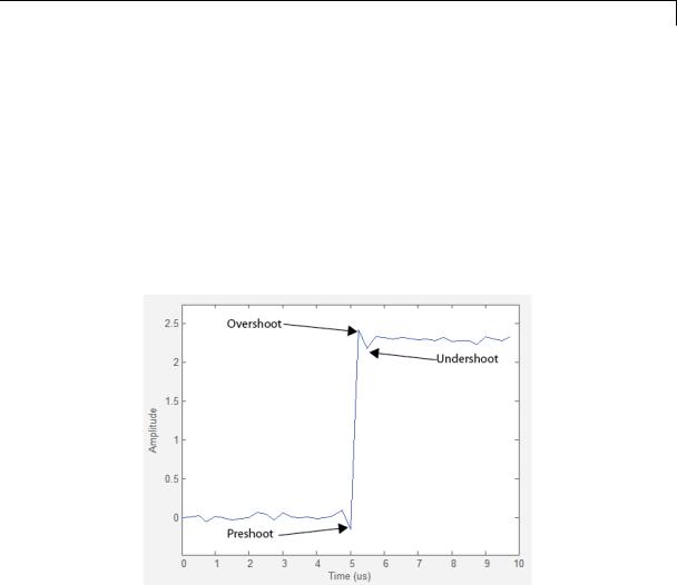
The Overshoots/Undershoots pane displays calculated measurements involving the distortion and damping of the input signal. Overshoot and undershoot refer to the amount that a signal respectively exceeds and falls below its final steady-state value. Preshoot refers to the amount prior to a transition that a signal varies from its initial steady-state value. This figure shows preshoot, overshoot, and undershoot for a rising-edge transition.

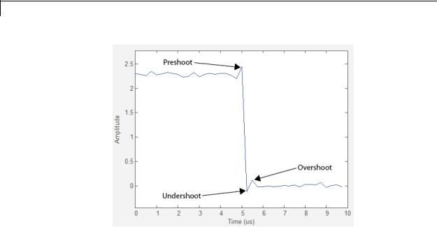
The next figure shows preshoot, overshoot, and undershoot for a falling-edge transition.

2-1781

Time Scope

•+ Preshoot — Average lowest aberration in the region immediately preceding each rising transition.

•+ Overshoot — Average highest aberration in the region immediately following each rising transition. For more information on the algorithm this measurement uses, see the Signal Processing Toolbox overshoot function reference.

•+ Undershoot — Average lowest aberration in the region immediately following each rising transition. For more information on the algorithm this measurement uses, see the Signal Processing Toolbox undershoot function reference.

•+ Settling Time — Average time required for each rising edge to enter and remain within the tolerance of the high-state level for the remainder of the settle seek duration. The settling time is the time after the mid-reference level instant when the signal crosses into and remains in the tolerance region around the high-state level. This crossing is illustrated in the following figure.

2-1782

Time Scope

You can modify the settle seek duration parameter in the Settings pane. For more information on the algorithm this measurement uses, see the Signal Processing Toolbox settlingtime function reference.

•– Preshoot — Average highest aberration in the region immediately preceding each falling transition.

•– Overshoot — Average highest aberration in the region immediately following each falling transition. For more information on the algorithm this measurement uses, see the Signal Processing Toolbox overshoot function reference.

•– Undershoot — Average lowest aberration in the region immediately following each falling transition. For more information on the algorithm this measurement uses, see the Signal Processing Toolbox undershoot function reference.

•– Settling Time — Average time required for each falling edge to enter and remain within the tolerance of the low-state level for the remainder of the settle seek duration. The settling time is the time after the mid-reference level instant when the signal crosses into and remains in the tolerance region around the low-state level. You can

2-1783

Time Scope

modify the settle seek duration parameter in the Settings pane. For more information on the algorithm this measurement uses, see the Signal Processing Toolbox settlingtime function reference.

Cycles

The Cycles pane displays calculated measurements pertaining to repetitions or trends in the displayed portion of the input signal.

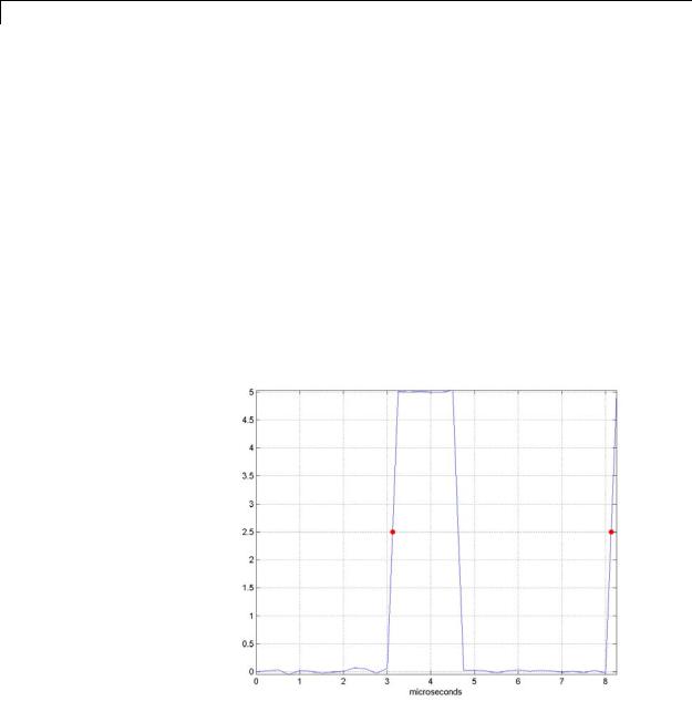
•Period — Average duration between adjacent edges of identical polarity within the displayed portion of the input signal. The Bilevel measurements panel calculates period as follows. It takes the difference between the mid-reference level instants of the initial transition of each positive-polarity pulse and the next positive-going transition. These mid-reference level instants appear as red dots in the following figure.

2-1784

Time Scope

For more information on the algorithm this measurement uses, see the Signal Processing Toolbox pulseperiod function reference.

•Frequency — Reciprocal of the average period. Whereas period is typically measured in some metric form of seconds, or seconds per cycle, frequency is typically measured in hertz or cycles per second.

•+ Pulses — Number of positive-polarity pulses counted.

•+ Width — Average duration between rising and falling edges of each positive-polarity pulse within the displayed portion of the input signal. For more information on the algorithm this measurement uses, see the Signal Processing Toolbox pulsewidth function reference.

•+ Duty Cycle — Average ratio of pulse width to pulse period for each positive-polarity pulse within the displayed portion of the input signal. For more information on the algorithm this measurement uses, see the Signal Processing Toolbox dutycycle function reference.

•– Pulses — Number of negative-polarity pulses counted.

•– Width — Average duration between rising and falling edges of each negative-polarity pulse within the displayed portion of the input signal. For more information on the algorithm this measurement uses, see the Signal Processing Toolbox pulsewidth function reference.

•– Duty Cycle — Average ratio of pulse width to pulse period for each negative-polarity pulse within the displayed portion of the input signal. For more information on the algorithm this measurement uses, see the Signal Processing Toolbox dutycycle function reference.

When you use the zoom options in the Scope, the bilevel measurements automatically adjust to the time range shown in the display. In the Scope toolbar, click the Zoom In or Zoom X button to constrict the x-axis range of the display, and the statistics shown reflect this time range. For example, you can zoom in on one rising edge to make the Bilevel Measurements panel display information about only that

2-1785