

- •Block Reference
- •Commonly Used
- •Continuous
- •Discontinuities
- •Discrete
- •Logic and Bit Operations
- •Lookup Tables
- •Math Operations
- •Model Verification
- •Model-Wide Utilities
- •Ports & Subsystems
- •Signal Attributes
- •Signal Routing
- •Sinks
- •Sources
- •User-Defined Functions
- •Additional Math & Discrete
- •Additional Discrete
- •Additional Math: Increment — Decrement
- •Run on Target Hardware
- •Target for Use with Arduino Hardware
- •Target for Use with BeagleBoard Hardware
- •Target for Use with LEGO MINDSTORMS NXT Hardware
- •Blocks — Alphabetical List
- •Command-Line Information
- •Command-Line Information
- •Command-Line Information
- •Command-Line Information
- •Command-Line Information
- •Command-Line Information
- •Command-Line Information
- •Command-Line Information
- •Command-Line Information
- •Command-Line Information
- •Command-Line Information
- •Command-Line Information
- •Command-Line Information
- •Command-Line Information
- •Command-Line Information
- •Command-Line Information
- •Settings Pane
- •Measurements Pane
- •Signal Statistics Measurements
- •Settings Pane
- •Transitions Pane
- •Overshoots/Undershoots
- •Cycles
- •Settings Pane
- •Peaks Pane
- •Command-Line Information
- •Command-Line Information
- •Command-Line Information
- •Command-Line Information
- •Command-Line Information
- •Command-Line Information
- •Command-Line Information
- •Command-Line Information
- •Command-Line Information
- •Function Reference
- •Model Construction
- •Simulation
- •Linearization and Trimming
- •Data Type
- •Examples
- •Main Toolbar
- •Command-Line Alternative
- •Command-Line Alternative
- •Command-Line Alternative
- •Command-Line Alternative
- •Command-Line Alternative
- •Command-Line Alternative
- •Mask Icon Drawing Commands
- •Simulink Classes
- •Model Parameters
- •About Model Parameters
- •Examples of Setting Model Parameters
- •Common Block Parameters
- •About Common Block Parameters
- •Examples of Setting Block Parameters
- •Block-Specific Parameters
- •Mask Parameters
- •About Mask Parameters
- •Notes on Mask Parameter Storage
- •Simulink Identifier
- •Simulink Identifier
- •Model Advisor Checks
- •Simulink Checks
- •Simulink Check Overview
- •See Also
- •Identify unconnected lines, input ports, and output ports
- •Description
- •Results and Recommended Actions
- •Capabilities and Limitations
- •Tips
- •See Also
- •Check root model Inport block specifications
- •Description
- •Results and Recommended Actions
- •See Also
- •Check optimization settings
- •Description
- •Results and Recommended Actions
- •Tips
- •See Also
- •Description
- •Results and Recommended Actions
- •See Also
- •Check for implicit signal resolution
- •Description
- •Results and Recommended Actions
- •See Also
- •Check for optimal bus virtuality
- •Description
- •Results and Recommended Actions
- •Capabilities and Limitations
- •See Also
- •Description
- •Results and Recommended Actions
- •Capabilities and Limitations
- •See Also
- •Identify disabled library links
- •Description
- •Results and Recommended Actions
- •Capabilities and Limitations
- •Tips
- •See Also
- •Identify parameterized library links
- •Description
- •Results and Recommended Actions
- •Capabilities and Limitations
- •Tips
- •See Also
- •Identify unresolved library links
- •Description
- •Results and Recommended Actions
- •Capabilities and Limitations
- •See Also
- •Results and Recommended Actions
- •Capabilities and Limitations
- •See Also
- •Results and Recommended Actions
- •Capabilities and Limitations
- •See Also
- •Check usage of function-call connections
- •Description
- •Results and Recommended Actions
- •See Also
- •Check signal logging save format
- •Description
- •Results and Recommended Actions
- •See Also
- •Description
- •Results and Recommended Actions
- •See Also
- •Description
- •Results and Recommended Actions
- •Tips
- •See Also
- •Check data store block sample times for modeling errors
- •Description
- •Results and Recommended Actions
- •See Also
- •Check for potential ordering issues involving data store access
- •Description
- •Results and Recommended Actions
- •Tips
- •See Also
- •Check for partial structure parameter usage with bus signals
- •Description
- •Results and Recommended Actions
- •Tips
- •See Also
- •Check for calls to slDataTypeAndScale
- •Description
- •Results and Recommended Actions
- •Tips
- •See Also
- •Check for proper bus usage
- •Description
- •Results and Recommended Actions
- •Action Results
- •Tips
- •See Also
- •Description
- •Results and Recommended Actions
- •See Also
- •Description
- •Results and Recommended Actions
- •See Also
- •Check for proper Merge block usage
- •Description
- •Input Parameters
- •Results and Recommended Actions
- •See Also
- •Description
- •Results and Recommended Actions
- •Action Results
- •See Also
- •Check for non-continuous signals driving derivative ports
- •Description
- •Results and Recommended Actions
- •See Also
- •Runtime diagnostics for S-functions
- •Description
- •Results and Recommended Actions
- •See Also
- •Check file for foreign characters
- •Description
- •Results and Recommended Actions
- •Tips
- •See Also
- •Check model for known block upgrade issues
- •Description
- •Results and Recommended Actions
- •Action Results
- •See Also
- •Description
- •Results and Recommended Actions
- •Action Results
- •See Also
- •Check that the model is saved in SLX format
- •Description
- •Results and Recommended Actions
- •Tips
- •See Also
- •Check Model History properties
- •Description
- •Results and Recommended Actions
- •See Also
- •Analyze model hierarchy for upgrade issues
- •Description
- •Results and Recommended Actions
- •Tips
- •See Also
- •Description
- •Results and Recommended Actions
- •See Also
- •Simulink Performance Advisor Checks
- •Simulink Performance Advisor Check Overview
- •See Also
- •Baseline
- •See Also
- •Check Preupdate Items
- •See Also
- •Checks that need Update Diagram
- •See Also
- •Checks that require simulation to run
- •See Also
- •Check Accelerator Settings
- •See Also
- •Create Baseline
- •See Also
- •Identify resource intensive diagnostic settings
- •See Also
- •Check optimization settings
- •See Also
- •Identify inefficient lookup table blocks
- •See Also
- •Identify Interpreted MATLAB Function blocks
- •See Also
- •Check MATLAB Function block debug settings
- •See Also
- •Check Stateflow block debug settings
- •See Also
- •Identify simulation target settings
- •See Also
- •Check model reference rebuild setting
- •See Also
- •Check Model Reference parallel build
- •See Also
- •Check solver type selection
- •See Also
- •Select normal or accelerator simulation mode
- •See Also
- •Simulink Limits
- •Maximum Size Limits of Simulink Models
- •Index
- •Filter Structures and Filter Coefficients
- •Valid Initial States
- •Number of Delay Elements (Filter States)
- •Frame-Based Processing
- •Sample-Based Processing
- •Valid Initial States
- •Frame-Based Processing
- •Sample-Based Processing
- •Model Parameters in Alphabetical Order
- •Common Block Parameters
- •Continuous Library Block Parameters
- •Discontinuities Library Block Parameters
- •Discrete Library Block Parameters
- •Logic and Bit Operations Library Block Parameters
- •Lookup Tables Block Parameters
- •Math Operations Library Block Parameters
- •Model Verification Library Block Parameters
- •Model-Wide Utilities Library Block Parameters
- •Ports & Subsystems Library Block Parameters
- •Signal Attributes Library Block Parameters
- •Signal Routing Library Block Parameters
- •Sinks Library Block Parameters
- •Sources Library Block Parameters
- •User-Defined Functions Library Block Parameters
- •Additional Discrete Block Library Parameters
- •Additional Math: Increment - Decrement Block Parameters
- •Mask Parameters

Switch
Allow different data input sizes
Select this check box to allow input signals with different sizes.
Settings
Default: Off
 On
On
Allows input signals with different sizes, and propagates the input signal size to the output signal. If the two data inputs are variable-size signals, the maximum size of the signals can be equal or different.
 Off
Off
Inputs signals must be the same size.
Command-Line Information
Parameter: AllowDiffInputSize
Type: string
Value: 'on' | 'off'
Default: 'off'
2-1718

Switch
Output minimum
Specify the minimum value that the block should output.
Settings
Default: []
The default value is [] (unspecified).
Simulink uses this value to perform:
•Parameter range checking (see “Check Parameter Values”) for some blocks
•Simulation range checking (see “Signal Ranges”)
•Automatic scaling of fixed-point data types
Tip
This number must be a finite real double scalar value.
Command-Line Information
See “Block-Specific Parameters” on page 8-109 for the command-line information.
2-1719

Switch
Output maximum
Specify the maximum value that the block should output.
Settings
Default: []
The default value is [] (unspecified).
Simulink uses this value to perform:
•Parameter range checking (see “Check Parameter Values”) for some blocks
•Simulation range checking (see “Signal Ranges”)
•Automatic scaling of fixed-point data types
Tip
This number must be a finite real double scalar value.
Command-Line Information
See “Block-Specific Parameters” on page 8-109 for the command-line information.
2-1720

Switch
Output data type
Specify the output data type.
Settings
Default: Inherit: Inherit via internal rule
Inherit: Inherit via internal rule
Uses the following rules to determine the output data type.
|
Data Type of First Input |
Output Data Type |
|
|
Port |
|
|
|
Has a larger positive range |
Inherited from the first input |
|
|
than the third input port |
port |
|
|
Has the same positive range |
Inherited from the third input |
|
|
as the third input port |
port |
|
|
Has a smaller positive range |
|
|
|
than the third input port |
|
|
Inherit: Inherit via back propagation
Uses data type of the driving block.
double
Specifies output data type is double.
single
Specifies output data type is single.
int8
Specifies output data type is int8.
uint8
Specifies output data type is uint8.
int16
Specifies output data type is int16.
uint16
Specifies output data type is uint16.
2-1721

Switch
int32
Specifies output data type is int32.
uint32
Specifies output data type is uint32.
fixdt(1,16,0)
Specifies output data type is fixed point fixdt(1,16,0).
fixdt(1,16,2^0,0)
Specifies output data type is fixed point fixdt(1,16,2^0,0).
Enum: <class name>
Uses an enumerated data type, for example, Enum: BasicColors.
<data type expression>
Uses a data type object, for example, Simulink.NumericType.
Tip
When the output is of enumerated type, both data inputs should use the same enumerated type as the output.
Command-Line Information
See “Block-Specific Parameters” on page 8-109 for the command-line information.
See Also
See “Specify Block Output Data Types” for more information.
2-1722
Switch
Mode
Select the category of data to specify.
Settings
Default: Inherit
Inherit
Specifies inheritance rules for data types. Selecting Inherit enables a list of possible values:
•Inherit via internal rule (default)
•Inherit via back propagation
Built in
Specifies built-in data types. Selecting Built in enables a list of possible values:
•double (default)
•single
•int8
•uint8
•int16
•uint16
•int32
•uint32
Fixed point
Specifies fixed-point data types.
Enumerated
Specifies enumerated data types. Selecting Enumerated enables you to enter a class name.
Expression
Specifies expressions that evaluate to data types. Selecting Expression enables you to enter an expression.
2-1723

Switch
Dependencies
Clicking the Show data type assistant button enables this parameter.
Command-Line Information
See “Block-Specific Parameters” on page 8-109 for the command-line information.
See Also
See “Specify Data Types Using Data Type Assistant”.
2-1724

Switch
Data type override
Specify data type override mode for this signal.
Settings
Default: Inherit
Inherit
Inherits the data type override setting from its context, that is, from the block, Simulink.Signal object or Stateflow chart in Simulink that is using the signal.
Off
Ignores the data type override setting of its context and uses the fixed-point data type specified for the signal.
Tip
The ability to turn off data type override for an individual data type provides greater control over the data types in your model when you apply data type override. For example, you can use this option to ensure that data types meet the requirements of downstream blocks regardless of the data type override setting.
Dependency
This parameter appears only when the Mode is Built in or Fixed point.
2-1725

Switch
Signedness
Specify whether you want the fixed-point data as signed or unsigned.
Settings
Default: Signed
Signed
Specifies the fixed-point data as signed.
Unsigned
Specifies the fixed-point data as unsigned.
Dependencies
Selecting Mode > Fixed point enables this parameter.
Command-Line Information
See “Block-Specific Parameters” on page 8-109 for the command-line information.
See Also
See “Specifying a Fixed-Point Data Type”.
2-1726

Switch
Word length
Specify the bit size of the word that holds the quantized integer.
Settings
Default: 16
Minimum: 0
Maximum: 32
Large word sizes represent large values with greater precision than small word sizes.
Dependencies
Selecting Mode > Fixed point enables this parameter.
Command-Line Information
See “Block-Specific Parameters” on page 8-109 for the command-line information.
See Also
See “Specifying a Fixed-Point Data Type” for more information.
2-1727

Switch
Scaling
Specify the method for scaling your fixed-point data to avoid overflow conditions and minimize quantization errors.
Settings
Default: Best precision
Binary point
Specify binary point location.
Slope and bias
Enter slope and bias.
Best precision
Specify best-precision values.
Dependencies
Selecting Mode > Fixed point enables this parameter. Selecting Binary point enables:
•Fraction length
•Calculate Best-Precision Scaling
Selecting Slope and bias enables:
•Slope
•Bias
•Calculate Best-Precision Scaling
Command-Line Information
See “Block-Specific Parameters” on page 8-109 for the command-line information.
See Also
For more information, see “Specifying a Fixed-Point Data Type”.
2-1728

Switch
Fraction length
Specify fraction length for fixed-point data type.
Settings
Default: 0
Binary points can be positive or negative integers.
Dependencies
Selecting Scaling > Binary point enables this parameter.
Command-Line Information
See “Block-Specific Parameters” on page 8-109 for the command-line information.
See Also
See “Specifying a Fixed-Point Data Type” for more information.
2-1729

Switch
Slope
Specify slope for the fixed-point data type.
Settings
Default: 2^0
Specify any positive real number.
Dependencies
Selecting Scaling > Slope and bias enables this parameter.
Command-Line Information
See “Block-Specific Parameters” on page 8-109 for the command-line information.
See Also
See “Specifying a Fixed-Point Data Type” for more information.
2-1730

Switch
Bus
Support
Bias
Specify bias for the fixed-point data type.
Settings
Default: 0
Specify any real number.
Dependencies
Selecting Scaling > Slope and bias enables this parameter.
Command-Line Information
See “Block-Specific Parameters” on page 8-109 for the command-line information.
See Also
See “Specifying a Fixed-Point Data Type” for more information.
The Switch block is a bus-capable block. The data inputs can be virtual or nonvirtual bus signals subject to the following restrictions:
•All the buses must be equivalent (same hierarchy with identical names and attributes for all elements).
•All signals in a nonvirtual bus input to a Switch block must have the same sample time. The requirement holds even if the elements of the associated bus object specify inherited sample times.
You can use a Rate Transition block to change the sample time of an individual signal, or of all signals in a bus. See “About Composite Signals” and Bus-Capable Blocks for more information.
You can use an array of buses as an input signal to a Switch block. For details about defining and using an array of buses, see “Combine Buses into an Array of Buses”. When using an array of buses with a Switch block, set the Threshold parameter to a scalar value.
2-1731
Switch
Examples Use of Boolean Input for the Control Port
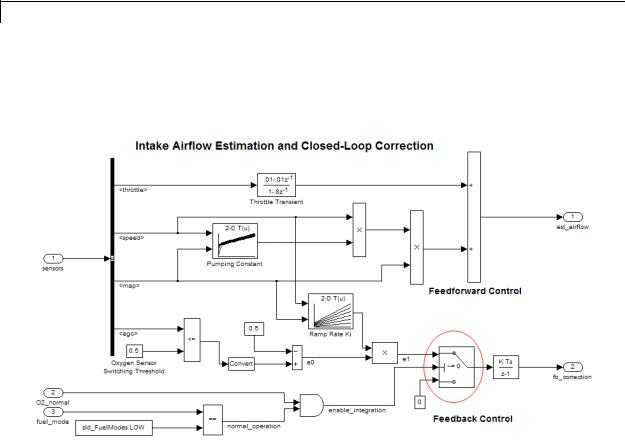
In the sldemo_fuelsys model, the fuel_rate_control/airflow_calc subsystem uses a Switch block:
The value of the control port on the Switch block determines whether or not feedback correction occurs. The control port value depends on the output of the Logical Operator block.
|
When the Logical |
The control port of |
And feedback |
|
|
Operator block |
the Switch block |
control... |
|
|
output is... |
is... |
|
|
|
TRUE |
1 |
Occurs |
|
|
FALSE |
0 |
Does not occur |
|
|
|
|
|
|
2-1732
Switch
Use of Simulation Time for the Control Port
The sldemo_zeroxing model uses a Switch block:
The value of the control port on the Switch block determines when the output changes from the first input to the third input.
|
When simulation time is... |
|
The Switch block output is... |
|
|
|
Less than or equal to 5 |
|
The first input from the Abs block |
|
|
|
Greater than 5 |
|
The third input from the |
|
|
|
|
|
|
Saturation block |
|
Characteristics |
|
|
|
|
|
Bus-capable |
|
Yes, with restrictions |
|
||
|
Direct Feedthrough |
|
Yes |
|
|
|
Sample Time |
|
Specified in the Sample time |
|
|
|
|
|
parameter |
|
|
|
Scalar Expansion |
|
Yes |
|
|
|
Dimensionalized |
|
Yes |
|
|
|
|
|
|
|
|
2-1733

Switch
|
|
Multidimensionalized |
Yes |
|
|
Zero-Crossing Detection |
Yes, if enabled |
See Also |
|
Multiport Switch |
|
2-1734
Switch Case
Purpose |
Implement C-like switch control flow statement |
Library |
Ports & Subsystems |
Description |
|
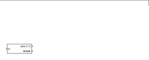
A Switch Case block receives a single input. Each output port is attached to a Switch Case Action subsystem. Data outputs are action signals to Switch Case Action subsystems, which you create with Action Port blocks and subsystems.
The Switch Case block uses its input value to select a case condition that determines which subsystem to execute. The cases are evaluated top down starting with the first case. If a case value (in brackets) corresponds to the value of the input, its Switch Case Action subsystem is executed.
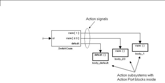
If a default case exists, it executes if none of the other cases executes. Providing a default case is optional, even if the other case conditions do not exhaust every possible value. The following diagram shows a completed Simulink switch control flow statement:
2-1735
Switch Case
Cases for the Switch Case block contain an implied break after their Switch Case Action subsystems are executed. Thus there is no fall-through behavior for the Simulink switch control flow statement as found in standard C switch statements. The following pseudocode represents generated code for the preceding switch control example:
switch (u1) { case [u1=1]:
body_1; break;
case [u1=2 or u1=3]: body_23;
break;
default: body_default;
}
To construct the Simulink switch control flow statement shown in the above example:
2-1736

Switch Case
1Place a Switch Case block in the current system and attach the input port labeled u1 to the source of the data you are evaluating.
2Open the Switch Case block dialog box and update parameters: a Populate the Case conditions field with the individual cases.
b To show a default case, select the Show default case check box.
3Create a Switch Case Action subsystem for each case port you added
to the Switch Case block.
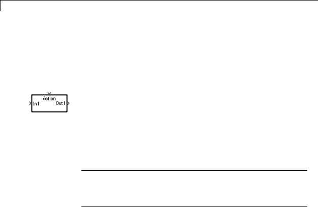
These consist of subsystems with Action Port blocks inside them. When you place the Action Port block inside a subsystem, the subsystem becomes an atomic subsystem with an input port labeled
Action.
4Connect each case output port and the default output port of the Switch Case block to the Action port of an Action subsystem.
Each connected subsystem becomes a case body. This is indicated by the change in label for the Switch Case Action subsystem block and the Action Port block inside of it to the name case{}.
During simulation of a switch control flow statement, the Action signals from the Switch Case block to each Switch Case Action subsystem turn from solid to dashed.
5In each Switch Case Action subsystem, enter the Simulink logic appropriate to the case it handles. All blocks in a Switch Case Action Subsystem must run at the same rate as the driving Switch Case block. You can achieve this by setting each block’s sample time parameter to be either inherited (-1) or the same value as the Switch Case block’s sample time.
Enumerated Types in Switch Case Blocks
The Switch Case block supports enumerated data types for the input signal and the case conditions. You specify enumerated case conditions
2-1737
Switch Case
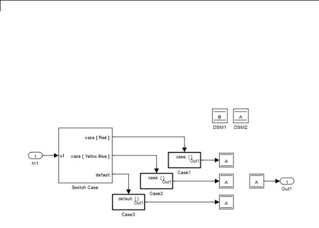
as a cell array of enumerated values in the Case conditions field, for example:
{BasicColors.Red, [BasicColors.Yellow, BasicColors.Blue]}
The Switch Case block icon shows the enumerated names that correspond to the case conditions, for example:
You can use the enumeration function to specify a case condition that includes a case for every value in an enumerated type. When you use enumerated data in a Switch Case block, follow these rules:
•If the input u1 is of an enumerated type, all case condition values must be of that same enumerated type.
•If any case condition value is of an enumerated type, the input u1 and all other case condition values must be of that same enumerated type.
•When the case condition values are of an enumerated type, each value that appears as a case condition must have a different underlying integer.
2-1738

Switch Case
Data Type
Support
For more information about enumerated data types in Simulink, see “Use Enumerated Data in Simulink Models”. The generated code for a Switch Case block that uses enumerated data uses the enumerated values of the specified case conditions, rather than their underlying integers.
The input to the port labeled u1 of a Switch Case block can be:
•A scalar value having a built-in data type that Simulink supports. The block does not support Boolean or fixed-point data types and truncates the numeric inputs to 32-bit signed integers.
•A scalar value of any enumerated data type, as described in “Enumerated Types in Switch Case Blocks” on page 2-1737.
For more information, see “Data Types Supported by Simulink” in the Simulink documentation.
2-1739
Switch Case
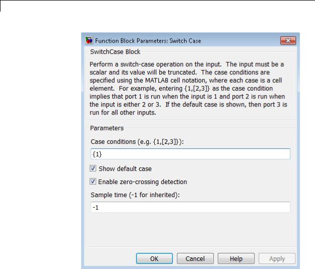
Parameters and Dialog Box
Case conditions
Specify the case conditions using MATLAB cell notation. For example, entering {1,[7,9,4]} specifies that output port case[1] is run when the input value is 1, and output port case[7 9 4] is run when the input value is 7, 9, or 4.
2-1740

Switch Case
You can use colon notation to specify a range of integer case conditions. For example, entering {[1:5]} specifies that output port case[1 2 3 4 5] is run when the input value is 1, 2, 3, 4, or 5.
Depending on block size, cases with long lists of conditions are displayed in shortened form in the Switch Case block, using a terminating ellipsis (...).
You can use the enumeration function to specify a case condition that includes a case for every value in an enumerated type.
Show default case
If you select this check box, the default output port appears as the last case on the Switch Case block, allowing you to specify a default case. This case executes when the input value does not match any of the case values specified in the Case conditions field. With Show default case selected, a default output port always appears, even if the preceding cases exhaust all possibilities for the input value.
Enable zero-crossing detection
Select to enable zero-crossing detection. For more information, see “Zero-Crossing Detection” in the Simulink documentation.
Sample time (-1 for inherited)
Specify the time interval between samples. To inherit the sample time, set this parameter to -1. See “Specify Sample Time” for more information.
Characteristics |
Direct Feedthrough |
Yes |
|
Sample Time |
Inherited from driving block |
|
Scalar Expansion |
No |
|
Dimensionalized |
No |
|
Zero-Crossing Detection |
Yes, if enabled |
|
|
|
2-1741
Switch Case Action Subsystem
Purpose |
Represent subsystem whose execution is triggered by Switch Case block |
Library |
Ports & Subsystems |
Description |
|
This block is a Subsystem block that is preconfigured to serve as a starting point for creating a subsystem whose execution is triggered by a Switch Case block.
Note All blocks in a Switch Case Action Subsystem must run at the same rate as the driving Switch Case block. You can achieve this by setting each block’s sample time parameter to be either inherited (-1) or the same value as the Switch Case block’s sample time.
For more information, see the Switch Case block and “Control Flow Logic” in the “Creating a Model” chapter of the Simulink documentation.
2-1742
Tapped Delay
Purpose |
Delay scalar signal multiple sample periods and output all delayed |
|
versions |
Library |
Discrete |
Description |
The Tapped Delay block delays an input by the specified number of |
|
sample periods and outputs all the delayed versions. Use this block to |
|
discretize a signal in time or resample a signal at a different rate. |
|
The block accepts one scalar input and generates an output vector that |
|
contains each delay. Specify the order of the delays in the output vector |
|
with the Order output vector starting with parameter: |
|
• Oldest orders the output vector starting with the oldest delay version |
|
and ending with the newest delay version. |
|
• Newest orders the output vector starting with the newest delay |
|
version and ending with the oldest delay version. |
|
Specify the output vector for the first sampling period with the Initial |
|
condition parameter. Careful selection of this parameter can minimize |
|
unwanted output behavior. |
|
Specify the time between samples with the Sample time parameter. |
|
Specify the number of delays with the Number of delays parameter. |
|
A value of -1 instructs the block to inherit the number of delays by back |
|
propagation. Each delay is equivalent to the z-1 discrete-time operator, |
|
which the Unit Delay block represents. |
Data Type The Tapped Delay block accepts signals of the following data types:
Support
•Floating point
•Built-in integer
•Fixed point
•Boolean
2-1743
Tapped Delay
For more information, see “Data Types Supported by Simulink” in the Simulink documentation.
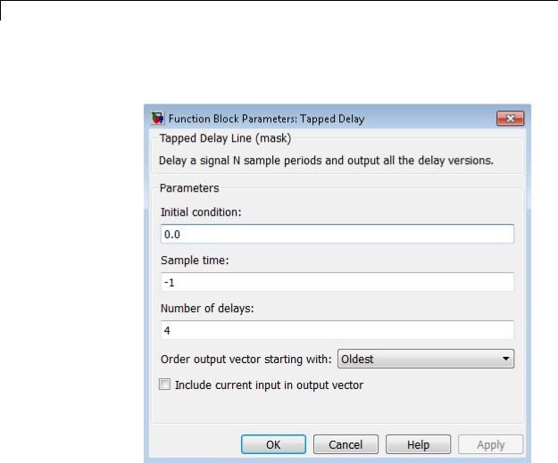
Parameters and Dialog Box
Initial condition
Specify the initial output of the simulation. The Initial condition parameter is converted from a double to the input data type offline using round-to-nearest and saturation. Simulink software does not allow you to set the initial condition of this block to inf or NaN.
2-1744

Tapped Delay
Sample time
Specify the time interval between samples. To inherit the sample time, set this parameter to -1. See “Specify Sample Time” in the online Simulink documentation for more information.
Number of delays
Specify the number of discrete-time operators.
Order output vector starting with
Specify whether to output the oldest delay version first, or the newest delay version first.
Include current input in output vector
Select to include the current input in the output vector.
Characteristics
See Also
Direct Feedthrough |
Yes, when Include current input in |
|
output vector check box is selected. |
|
No, otherwise. |
Sample Time |
Specified in the Sample time |
|
parameter |
Scalar Expansion |
Yes, of initial conditions |
|
|
Unit Delay
2-1745
Terminator
Purpose |
Terminate unconnected output port |
Library Sinks
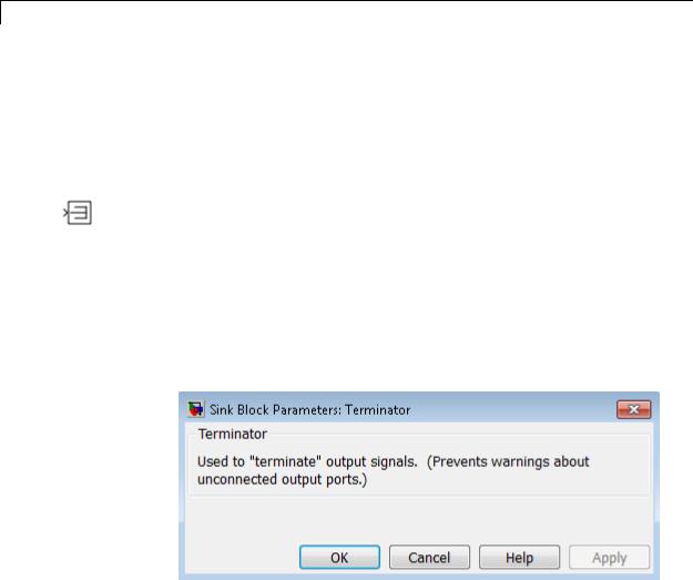
Description Use the Terminator block to cap blocks whose output ports do not connect to other blocks. If you run a simulation with blocks having unconnected output ports, Simulink issues warning messages. Using Terminator blocks to cap those blocks helps prevent warning messages.
Data Type The Terminator block accepts real or complex signals of any data type
Support that Simulink supports, including fixed-point and enumerated data types.
For more information, see “Data Types Supported by Simulink” in the Simulink documentation.
Parameters and Dialog Box
Examples |
The following Simulink examples show how to use the Terminator block: |
|
• sldemo_bounce |
2-1746

Terminator
• sldemo_fuelsys
• aero_six_dof
Characteristics |
Sample Time |
Inherited from the driving block |
|
Dimensionalized |
Yes |
|
Multidimensionalized |
Yes |
|
Virtual |
Yes |
|
|
For more information, see “Virtual |
|
|
Blocks” in the Simulink documentation. |
|
Zero-Crossing Detection |
No |
|
|
|
2-1747

Timed-Based Linearization
Purpose
Library
Description
Generate linear models in base workspace at specific times
Model-Wide Utilities
This block calls linmod or dlinmod to create a linear model for the system when the simulation clock reaches the time specified by the Linearization time parameter. No trimming is performed. The linear model is stored in the base workspace as a structure, along with information about the operating point at which the snapshot was taken. Multiple snapshots are appended to form an array of structures.
The block sets the following model parameters to the indicated values:
•BufferReuse = 'off'
•RTWInlineParameters = 'on'
•BlockReductionOpt = 'off'
The name of the structure used to save the snapshots is the name of the model appended by _Timed_Based_Linearization, for example, vdp_Timed_Based_Linearization. The structure has the following fields:
|
Field |
Description |
|
|
a |
The A matrix of the linearization |
|
|
b |
The B matrix of the linearization |
|
|
c |
The C matrix of the linearization |
|
|
d |
The D matrix of the linearization |
|
|
StateName |
Names of the model’s states |
|
|
OutputName |
Names of the model’s output ports |
|
|
InputName |
Names of the model’s input ports |
|
|
|
|
|
2-1748

Timed-Based Linearization
|
Field |
Description |
|
|
OperPoint |
A structure that specifies the operating point |
|
|
|
of the linearization. The structure specifies the |
|
|
|
operating point time (OperPoint.t). The states |
|
|
|
(OperPoint.x) and inputs (OperPoint.u) fields |
|
|
|
are not used. |
|
|
Ts |
The sample time of the linearization for a discrete |
|
|
|
linearization |
|
Use the Trigger-Based Linearization block if you need to generate linear models conditionally.
You can use state and simulation time logging to extract the model states and inputs at operating points. For example, suppose that you want to get the states of the f14 example model at linearization times of 2 seconds and 5 seconds.
1 Open the model and drag an instance of this block from the Model-Wide Utilities library and drop the instance into the model.
2Open the block’s parameter dialog box and set the Linearization time to 2 and 5.
3Open the model’s Model Configuration Parameters dialog box.
4Select the Data Import/Export pane.
5Check States and Time on the Save to Workspace control panel
6Select OK to confirm the selections and close the dialog box.
7Simulate the model.
At the end of the simulation, the following variables appear in the MATLAB workspace: f14_Timed_Based_Linearization, tout, and xout.
2-1749

Timed-Based Linearization
Data Type
Support
8Get the indices to the operating point times by entering the following at the MATLAB command line:
ind1 = find(f14_Timed_Based_Linearization(1).OperPoint.t==tout);
ind2 = find(f14_Timed_Based_Linearization(1).OperPoint.t==tout);
9Get the state vectors at the operating points.
x1 = xout(ind1,:);
x2 = xout(ind2,:);
Not applicable.
2-1750
Timed-Based Linearization
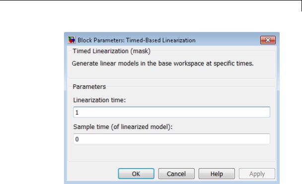
Parameters and
Dialog |
Linearization time |
|
Box |
Time at which you want the block to generate a linear model. |
|
Enter a vector of times if you want the block to generate linear |
||
|
||
|
models at more than one time step. |
Sample time (of linearized model)
Specify a sample time to create discrete-time linearizations of the model (see “Discrete-Time System Linearization” on page 4-21).
Characteristics |
|
Sample Time |
Specified in the Sample time |
|
|
|
parameter |
|
|
Dimensionalized |
No |
See Also |
|
Trigger-Based Linearization |
|
2-1751
Time Scope
Purpose |
Display time-domain signals |
Description The Time Scope block displays signals in the time domain. The Time Scope block accepts input signals with the following characteristics:
•Continuous or discrete sample time
•Realor complex-valued
•Fixed or variable size dimensions
•Floatingor fixed-point data type
•N-dimensional
•Simulink enumerations
2-1752
Time Scope
You can use the Time Scope block in models running in Normal or Accelerator simulation modes. You can also use the Time Scope block in models running in Rapid Accelerator or External simulation modes, with some limitations. See the “Supported Simulation Modes” on page 2-1822 section for more information.
You can use the Time Scope block inside of all subsystems and conditional subsystems. Conditional subsystems include enabled subsystems, triggered subsystems, enabled and triggered subsystems, and function-call subsystems. See “About Conditional Subsystems” in the Simulink documentation for more information.
2-1753

Time Scope
|
See the following sections for more information on the Time Scope: |
|
|
• “Displaying Multiple Signals” on page 2-1754 |
|
|
• “Signal Display” on page 2-1757 |
|
|
• “Toolbar” on page 2-1761 |
|
|
• “Simulation Toolbar” on page 2-1764 |
|
|
• “Measurements Panels” on page 2-1766 |
|
|
• “Properties Dialog Box” on page 2-1789 |
|
|
• “Style Dialog Box” on page 2-1800 |
|
|
• “Simulation Stepping Options” on page 2-1803 |
|
|
• “Core — General UI Options” on page 2-1805 |
|
|
• “Visuals — Time Domain Options” on page 2-1808 |
|
|
• “Tools — Plot Navigation Options” on page 2-1817 |
|
|
• “Sources — Simulink Options” on page 2-1821 |
|
|
• “Supported Data Types” on page 2-1821 |
|
|
• “Supported Simulation Modes” on page 2-1822 |
|
Displaying |
Multiple Signal Input |
|
Multiple |
You can configure the Time Scope block to show multiple signals within |
|
Signals |
||
the same display or on separate displays. By default, the signals appear |
||
|
as different-colored lines on the same display. The signals can have |
|
|
different dimensions, sample rates, and data types. Each signal can be |
|
|
either real or complex valued. You can set the number of input ports |
|
|
on the Time Scope block in the following ways: |
|
|
• Right-click the Time Scope block in your model to bring up the |
|
|
context menu. Point your cursor to the Signals & Ports > Number |
|
|
of Input Ports item on the context menu. You can then select |
|
|
the number of input ports for the Time Scope block. If the desired |
|
|
number of input signals is 1, 2, or 3, then click on the appropriate |
2-1754

Time Scope
value. To configure a Time Scope block to have more than three input ports, select More, and enter a number for the Number of input ports parameter.
•Open the Time Scope window by double-clicking the Time Scope block in your model. To specify how many input ports the Time Scope block should have, in the Time Scope menu, select File > Number of Input Ports from the scope menu.
An input signal may contain multiple channels, depending on its dimensions. Multiple channels of data are always shown as different-colored lines on the same display.
Multiple Time Offsets
You can offset all channels of an input signal by the same number of seconds or offset each channel independently. To offset all channels equally, select View > Properties, and specify a scalar value for the Time display offset parameter on the Main pane. To offset each channel independently, specify a vector of offset values. When you specify a Time display offset vector of length N, the scope offsets the input channels as follows:
•When N is equal to the number of input channels, the scope offsets each channel according to its corresponding value in the offset vector.
•When N is less than the number of input channels, the scope applies the values you specify in the offset vector to the first N input channels. The scope does not offset the remaining channels.
•When N is greater than the number of input channels, the scope offsets each input channel according to the corresponding value in the offset vector. The scope ignores all values in the offset vector that do not correspond to a channel of the input.
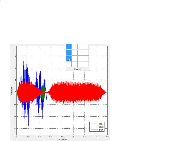
Multiple Displays
You can display multiple channels of data on different displays in the Scope window. In the Scope toolbar, select View > Layout, or select
the Layout button ( ). This feature allows you to tile the window into
2-1755
Time Scope
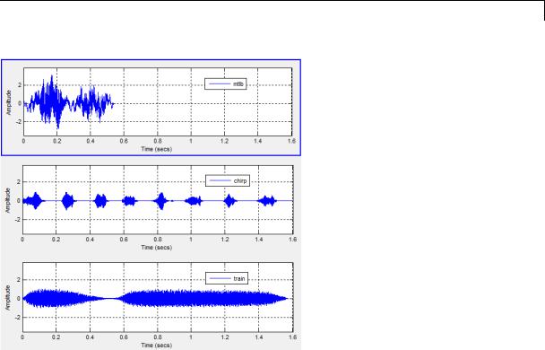
a number of separate displays, up to a grid of 4 rows and 4 columns. For example, if there are three inputs to the Scope, you can display the signals in separate displays by selecting row 3, column 1, as shown in the following figure.
After you select row 3, column 1, the Scope window has three separate displays, as shown in the following figure.
2-1756
Time Scope
Signal |
Time Scope uses the simulation start time and stop time in order to |
Display |
determine the default time range. However, you can define the length |
|
of simulation time for which the Time Scope displays data. To change |
|
the signal display settings, select View > Properties to bring up the |
|
Properties dialog box. Then, modify the values for the Time span and |
|
Time display offset parameters on the Time tab. For example, if you |
|
set the Time span to 20 seconds and the Time display offset to 0, |
|
the scope displays 20 seconds’ worth of simulation data at a time. The |
|
values on the time-axis of the Time Scope display remain the same |
|
throughout simulation. |
|
To communicate the simulation time that corresponds to the current |
|
display, the scope uses the Time units, Time offset, and Simulation |
|
time indicators on the scope window. The following figure highlights |
|
these and other important aspects of the Time Scope window. |
2-1757
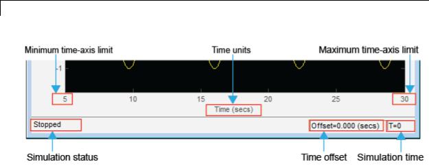
Time Scope
•Minimum time-axis limit — The Time Scope sets the minimum time-axis limit using the value of the Time display offset parameter on the Time tab of the Properties dialog box. If you specify a vector of values for the Time display offset parameter, the scope uses the smallest of those values to set the minimum time-axis limit.
•Maximum time-axis limit — The Time Scope sets the maximum time-axis limit by summing the value of Time display offset parameter with the value of the Time span parameter. If you specify a vector of values for the Time display offset parameter, the scope sets the maximum time-axis limit by summing the largest of those values with the value of the Time span parameter.
•Simulation status — Provides the current status of the model simulation. The status can be one of the following conditions:
-Initializing
-Ready
-Running
-Paused
The Simulation status is part of the Status Bar in the Time Scope window. You can choose to hide or display the entire Status Bar. From the Time Scope menu, select View > Status Bar.
2-1758

Time Scope
•Time units — The units used to describe the time-axis. The Time Scope sets the time units using the value of the Time Units parameter on the Time tab of the Properties dialog box. By default,
this parameter is set to Metric (based on Time Span) and displays in metric units such as milliseconds, microseconds, minutes, days, etc. You can change it to Seconds to always display the time-axis values in units of seconds. You can change it to None to not display any units on the time-axis. When you set this parameter to None, then Time Scope shows only the word Time on the time-axis.
To hide both the word Time and the values on the time-axis, set the Show time-axis labels parameter to None. To hide both the word Time and the values on the time-axis in all displays except the
bottom ones in each column of displays, set this parameter to Bottom Displays Only. This behavior differs from the Simulink Scope block, which always shows the values but never shows a label on the x-axis.
•Time offset — The Time offset value helps you determine the simulation times for which the scope is displaying data. The value is always in the range 0≤ Time offset≤ Simulation time.
For example, if you set the Time span to 20 seconds, and you see a Time offset of 0 (secs) on the scope window, the scope is displaying data for the first 0 to 20 seconds of simulation time. When you see the Time offset change to 20 (secs), the scope is
displaying data for simulation times is greater than 20 seconds and less than or equal to 40 seconds. The scope continues to update the Time offset value until the simulation is complete.
•Simulation time — When the model is running or simulation has been paused, the scope displays the current simulation time. If the model simulation completes or is stopped, the scope displays the time at which the simulation stopped. The Simulation time is part of the Status Bar in the Time Scope window. You can choose to hide or display the entire Status Bar. From the Time Scope menu, select
View > Status Bar .
2-1759

Time Scope
Axes Maximization
You can specify whether to display the Time Scope in maximized axes mode. In this mode, the axes are expanded to fill the entire display. To conserve space, no labels appear in each display. Instead, tick-mark values appear on top of the plotted data. The following figure highlights the important indicators in this mode of the Time Scope window.
To toggle this mode, in the Time Scope menu, select View > Properties to bring up the Properties dialog box. In the Main pane, set the Maximize axes parameter. You can select one of the following options:
•Auto — In this mode, the axes appear maximized in all displays only if the Title and Y-Axis label parameters are empty for every display. If you enter any value in any display for either of these parameters, the axes are not maximized.
•On — In this mode, the axes appear maximized in all displays. Any values entered into the Title and Y-Axis label parameters are hidden.
•Off — In this mode, none of the axes appear maximized.
The default setting is Auto.
Reduce Updates to Improve Performance
By default, the Time Scope updates the displays periodically at a rate not exceeding 20 hertz. If you would like the Time Scope to update on every simulation time step, you can disable the Reduce Updates to Improve Performance option. In the Time Scope menu, select
2-1760

Time Scope
Simulation > Reduce Updates to Improve Performance to clear the check box. However, as a recommended practice, you can leave this option enabled because doing so can significantly improve the speed of the simulation.
Toolbar |
The Time Scope toolbar contains the following buttons. |
|||
|
Print and Properties Buttons |
|||
|
|
|
|
|
|
ButtonMenu |
Shortcut |
Description |
|
|
|
Location |
Keys |
|
|
|
File > |
Ctrl+P |
Print the current scope window. |
|
|
|
Printing is available only when the |
|
|
|
|
|
scope display is not changing. You can |
|
|
|
|
enable printing by placing the scope |
|
|
|
|
in snapshot mode, pausing or stopping |
|
|
|
|
model simulation, or simulating the |
|
|
|
|
model in step-forward mode. |
|
|
|
|
To print the current scope window to |
|
|
|
|
a figure rather than sending it to your |
|
|
|
|
printer, select File > Print to figure. |
|
|
View > |
N/A |
Open the Properties dialog box. |
|
|
Properties |
|
See the “Properties Dialog Box” |
|
|
|
|
|
|
|
|
|
on page 2-1789 section for more |
|
|
|
|
information. |
2-1761

Time Scope
Axes Control Buttons
|
Tools > |
N/A |
When this tool is active, you can zoom |
|
Zoom In |
|
in on the scope window. To do so, click |
|
|
|
in the center of your area of interest, |
|
|
|
or click and drag your cursor to draw |
|
|
|
a rectangular area of interest inside |
|
|
|
the scope window. |
|
Tools > |
N/A |
When this tool is active, you can zoom |
|
Zoom X |
|
in on the x-axis. To do so, click inside |
|
|
|
the scope window, or click and drag |
|
|
|
your cursor along the x-axis over your |
|
|
|
area of interest. |
|
Tools > |
N/A |
When this tool is active, you can zoom |
|
Zoom Y |
|
in on the y-axis. To do so, click inside |
|
|
|
the scope window, or click and drag |
|
|
|
your cursor along the y-axis over your |
|
|
|
area of interest. |
|
Tools > |
Ctrl+A |
Click this button to scale the axes in |
|
Scale Axes |
|
the active scope window. |
|
Limits |
|
Alternatively, you can enable |
|
|
|
|
|
|
|
automatic axes scaling by selecting |
|
|
|
one of the following options from the |
|
|
|
Tools menu: |
|
|
|
• Automatically Scale Axes Limits |
|
|
|
— When you select this option, the |
|
|
|
scope scales the axes as needed |
|
|
|
during simulation. |
|
|
|
• Scale Axes Limits at Stop — |
|
|
|
When you select this option, the |
|
|
|
scope scales the axes each time the |
|
|
|
simulation is stopped. |
2-1762
Time Scope
Measurements Buttons
|
Tools > |
N/A |
Open or close the Cursor |
|
Measurements |
> |
Measurements panel. This |
|
Cursor |
|
panel puts screen cursors on all the |
|
Measurements |
|
displays. |
|
|
|
See the “Cursor Measurements Panel” |
|
|
|
on page 2-1768 section for more |
|
|
|
information. |
|
Tools > |
N/A |
Open or close the Signal Statistics |
|
Measurements |
> |
panel. This panel displays the |
|
Signal |
|
maximum, minimum, peak-to-peak |
|
Statistics |
|
difference, mean, median, RMS values |
|
|
|
of a selected signal, and the times at |
|
|
|
which the maximum and minimum |
|
|
|
occur. |
|
|
|
See the “Signal Statistics Panel” |
|
|
|
on page 2-1770 section for more |
|
|
|
information. |
|
Tools > |
N/A |
Open or close the Bilevel |
|
Measurements |
> |
Measurements panel. This panel |
|
Bilevel |
|
displays information about a selected |
|
Measurements |
|
signal’s transitions, overshoots or |
|
|
|
undershoots, and cycles. |
|
|
|
See the “Bilevel Measurements Panel” |
|
|
|
on page 2-1772 section for more |
|
|
|
information. |
|
Tools > |
N/A |
Open or close the Peak Finder panel. |
|
Measurements |
> |
This panel displays maxima and the |
|
Peak |
|
times at which they occur, allowing |
|
Finder |
|
the settings for peak threshold, |
|
|
|
maximum number of peaks, and peak |
|
|
|
excursion to be modified. |
2-1763

Time Scope
|
|
|
|
|
|
See the “Peak Finder Panel” on page |
|
|
|
|
|
|
|
|
2-1786 section for more information. |
|
|
|
|
Other Buttons |
|
|
|
|
|
|
|
|
|
|
|
|
|
|
|
|
|
|
View > |
|
N/A |
Arrange the layout of displays in the |
|
|
|
|
|
Layout |
|
|
Time Scope. This feature allows you |
|
|
|
|
|
|
|
|
to tile your screen into a number of |
|
|
|
|
|
|
|
|
separate displays, up to a grid of 4 |
|
|
|
|
|
|
|
|
rows and 4 columns. You may find |
|
|
|
|
|
|
|
|
multiple displays useful when the |
|
|
|
|
|
|
|
|
Time Scope takes multiple input |
|
|
|
|
|
|
|
|
signals. The default display is 1 row |
|
|
|
|
|
|
|
|
and 1 column. See the “Multiple |
|
|
|
|
|
|
|
|
Displays” on page 2-1755 section for |
|
|
|
|
|
|
|
|
more information. |
|
|
|
|
You can control whether this toolbar appears in the Time Scope window. |
|
|||||
|
|
From the Time Scope menu, select View > Toolbar. |
|
|||||
Simulation |
The Simulation Toolbar contains the following buttons. |
|
||||||
Toolbar |
|
|
|
|
|
|
|
|
|
ButtonMenu |
|
Shortcut |
Description |
|
|||
|
|
|
|
|||||
|
|
|
Location |
|
Keys |
|
|
|
|
|
|
Simulation > |
|
N/A |
|
Open the Simulation Stepping |
|
|
|
|
Simulation |
|
|
|
Options dialog box. This button |
|
|
|
|
Stepping |
|
|
|
appears only when you have |
|
|
|
|
Options |
|
|
|
previous stepping disabled. See |
|
|
|
|
|
|
|
|
the “Simulation Stepping Options” |
|
|
|
|
|
|
|
|
|
|
2-1764
Time Scope
ButtonMenu |
Shortcut |
Description |
|
|
Location |
Keys |
|
|
|
|
|
|
|
|
on page 2-1803 section for more |
|
|
|
information. |
|
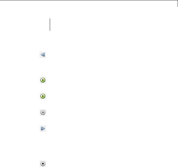
Simulation > |
N/A |
Advance the model simulation |
|
Previous |
|
backward by one time step. This |
|
Step |
|
button appears only when you have |
|
|
|
previous stepping enabled and the |
|
|
|
model simulation is paused. |
|
Simulation > |
Ctrl+T, |
Start the model simulation. This |
|
Run |
p, |
button appears only when the |
|
|
Space |
model simulation is stopped. |
|
Simulation > |
p, |
Continue the model simulation. |
|
Continue |
Space |
This button appears only when the |
|
|
|
model simulation is paused. |
|
Simulation > |
p, |
Pause the model simulation. This |
|
Pause |
Space |
button appears only when the |
|
|
|
model simulation is running. |
|
Simulation > |
Right |
Advance the model simulation |
|
Step |
arrow, |
forward by one time step. This |
|
Forward |
Page |
button starts the model simulation, |
|
|
Down |
allows it to run for one time step, |
|
|
|
and then pauses it again. The |
|
|
|
scope window then updates with |
|
|
|
the latest data. |
|
Simulation > |
Ctrl+T, |
Stop the model simulation. This |
|
Stop |
s |
button appears only when the |
|
|
|
model simulation is running or |
|
|
|
paused. |
2-1765

Time Scope
Measurements
Panels
|
ButtonMenu |
Shortcut |
Description |
|
|
|
|
Location |
Keys |
|
|
|
|
Simulation > |
N/A |
Take a snapshot of the current |
|
|
|
Simulink |
|
scope display. This button |
|
|
|
Snapshot |
|
temporarily freezes the scope |
|
|
|
|
|
display, while allowing simulation |
|
|
|
|
|
to continue running. To unfreeze |
|
|
|
|
|
the scope display and view the |
|
|
|
|
|
current simulation data, toggle this |
|
|
|
|
|
button to turn off snapshot mode. |
|
|
|
View > |
Ctrl+L |
Bring the model window forward, |
|
|
|
Highlight |
|
and highlight the Time Scope block |
|
|
|
Simulink |
|
whose display you are currently |
|
|
|
Block |
|
viewing. The Time Scope block |
|
|
|
|
|
that corresponds to the active Time |
|
|
|
|
|
Scope window flashes three times |
|
|
|
|
|
in the model. |
|
You can control whether this toolbar appears in the Time Scope window. From the Time Scope menu, select View > Simulation Toolbar.
To see a full listing of the shortcut keys for these simulation controls, from the Time Scope menu, select Help > Keyboard Command Help.
The Measurements panels are the five panels that appear to the right side of the Time Scope GUI. These panels are labeled Trace selection,
Signal statistics, Bilevel measurements, and Peak finder.
The Time Domain Measurements panels only appear if the Measurements tool is enabled in the Time Scope — Tools:Plot Navigation Options dialog box. To open this dialog box, in the Time Scope menu, select File > Configuration and click the Tools pane. If you disable the tool by clearing the Enabled check box, the Time Domain Measurements tools no longer display in the Time Scope GUI. You can reenable the tool at any time by selecting the Enabled check
2-1766
Time Scope
box. See the “Tools — Plot Navigation Options” on page 2-1817 section for more information.
Measurements Panel Buttons
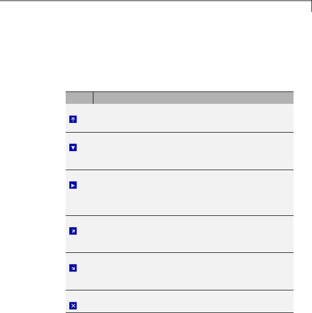
Each of the Measurements panels contains the following buttons that enable you to modify the appearance of the current panel.
Button Description
Move the current panel to the top. When you are displaying more than one panel, this action moves the current panel above all the other panels.
Collapse the current panel. When you first enable a panel, by default, it displays one or more of its panes. Click this button to hide all of its panes to conserve space. After you click this
button, it becomes the expand button  .
.
Expand the current panel. This button appears after you click the collapse button to hide the panes in the current panel. Click this button to display the panes in the current panel and show measurements again. After you click this
button, it becomes the collapse button  again.
Undock the current panel. This button lets you move the current panel into a separate window that can be relocated anywhere on your screen. After you click this button, it
becomes the dock button  in the new window.
Dock the current panel. This button appears only after you click the undock button. Click this button to put the current panel back into the right side of the Scope window. After you
click this button, it becomes the undock button  again.
Close the current panel. This button lets you remove the current panel from the right side of the Scope window.
Some panels have their measurements separated by category into a number of panes. Click the pane expand button  to show each pane
2-1767
Time Scope
that is hidden in the current panel. Click the pane collapse button  to hide each pane that is shown in the current panel.
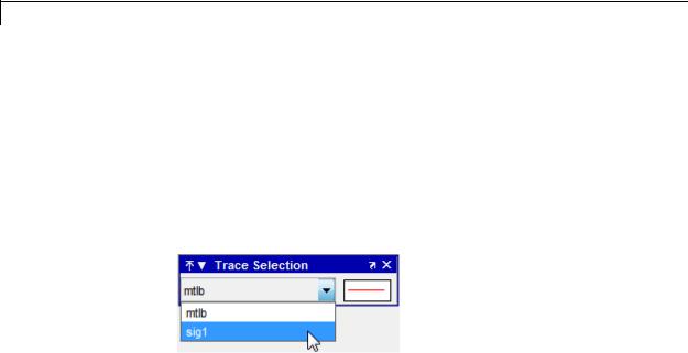
Trace Selection Panel
When you use the Scope to view multiple signals, the Trace Selection panel appears if you have more than one signal displayed and you click on any of the other Measurements panels. Choose the signal name for which you would like to display time domain measurements. See the following figure.
You can choose to hide or display the Trace Selection panel. In the Scope menu, select Tools > Measurements > Trace Selection.
Cursor Measurements Panel
The Cursor Measurements panel displays screen cursors. You can choose to hide or display the Cursor Measurements panel. In the Scope menu, select Tools > Measurements > Cursor
Measurements. Alternatively, in the Scope toolbar, click the Cursor Measurements  button.
2-1768