

- •Block Reference
- •Commonly Used
- •Continuous
- •Discontinuities
- •Discrete
- •Logic and Bit Operations
- •Lookup Tables
- •Math Operations
- •Model Verification
- •Model-Wide Utilities
- •Ports & Subsystems
- •Signal Attributes
- •Signal Routing
- •Sinks
- •Sources
- •User-Defined Functions
- •Additional Math & Discrete
- •Additional Discrete
- •Additional Math: Increment — Decrement
- •Run on Target Hardware
- •Target for Use with Arduino Hardware
- •Target for Use with BeagleBoard Hardware
- •Target for Use with LEGO MINDSTORMS NXT Hardware
- •Blocks — Alphabetical List
- •Command-Line Information
- •Command-Line Information
- •Command-Line Information
- •Command-Line Information
- •Command-Line Information
- •Command-Line Information
- •Command-Line Information
- •Command-Line Information
- •Command-Line Information
- •Command-Line Information
- •Command-Line Information
- •Command-Line Information
- •Command-Line Information
- •Command-Line Information
- •Command-Line Information
- •Command-Line Information
- •Settings Pane
- •Measurements Pane
- •Signal Statistics Measurements
- •Settings Pane
- •Transitions Pane
- •Overshoots/Undershoots
- •Cycles
- •Settings Pane
- •Peaks Pane
- •Command-Line Information
- •Command-Line Information
- •Command-Line Information
- •Command-Line Information
- •Command-Line Information
- •Command-Line Information
- •Command-Line Information
- •Command-Line Information
- •Command-Line Information
- •Function Reference
- •Model Construction
- •Simulation
- •Linearization and Trimming
- •Data Type
- •Examples
- •Main Toolbar
- •Command-Line Alternative
- •Command-Line Alternative
- •Command-Line Alternative
- •Command-Line Alternative
- •Command-Line Alternative
- •Command-Line Alternative
- •Mask Icon Drawing Commands
- •Simulink Classes
- •Model Parameters
- •About Model Parameters
- •Examples of Setting Model Parameters
- •Common Block Parameters
- •About Common Block Parameters
- •Examples of Setting Block Parameters
- •Block-Specific Parameters
- •Mask Parameters
- •About Mask Parameters
- •Notes on Mask Parameter Storage
- •Simulink Identifier
- •Simulink Identifier
- •Model Advisor Checks
- •Simulink Checks
- •Simulink Check Overview
- •See Also
- •Identify unconnected lines, input ports, and output ports
- •Description
- •Results and Recommended Actions
- •Capabilities and Limitations
- •Tips
- •See Also
- •Check root model Inport block specifications
- •Description
- •Results and Recommended Actions
- •See Also
- •Check optimization settings
- •Description
- •Results and Recommended Actions
- •Tips
- •See Also
- •Description
- •Results and Recommended Actions
- •See Also
- •Check for implicit signal resolution
- •Description
- •Results and Recommended Actions
- •See Also
- •Check for optimal bus virtuality
- •Description
- •Results and Recommended Actions
- •Capabilities and Limitations
- •See Also
- •Description
- •Results and Recommended Actions
- •Capabilities and Limitations
- •See Also
- •Identify disabled library links
- •Description
- •Results and Recommended Actions
- •Capabilities and Limitations
- •Tips
- •See Also
- •Identify parameterized library links
- •Description
- •Results and Recommended Actions
- •Capabilities and Limitations
- •Tips
- •See Also
- •Identify unresolved library links
- •Description
- •Results and Recommended Actions
- •Capabilities and Limitations
- •See Also
- •Results and Recommended Actions
- •Capabilities and Limitations
- •See Also
- •Results and Recommended Actions
- •Capabilities and Limitations
- •See Also
- •Check usage of function-call connections
- •Description
- •Results and Recommended Actions
- •See Also
- •Check signal logging save format
- •Description
- •Results and Recommended Actions
- •See Also
- •Description
- •Results and Recommended Actions
- •See Also
- •Description
- •Results and Recommended Actions
- •Tips
- •See Also
- •Check data store block sample times for modeling errors
- •Description
- •Results and Recommended Actions
- •See Also
- •Check for potential ordering issues involving data store access
- •Description
- •Results and Recommended Actions
- •Tips
- •See Also
- •Check for partial structure parameter usage with bus signals
- •Description
- •Results and Recommended Actions
- •Tips
- •See Also
- •Check for calls to slDataTypeAndScale
- •Description
- •Results and Recommended Actions
- •Tips
- •See Also
- •Check for proper bus usage
- •Description
- •Results and Recommended Actions
- •Action Results
- •Tips
- •See Also
- •Description
- •Results and Recommended Actions
- •See Also
- •Description
- •Results and Recommended Actions
- •See Also
- •Check for proper Merge block usage
- •Description
- •Input Parameters
- •Results and Recommended Actions
- •See Also
- •Description
- •Results and Recommended Actions
- •Action Results
- •See Also
- •Check for non-continuous signals driving derivative ports
- •Description
- •Results and Recommended Actions
- •See Also
- •Runtime diagnostics for S-functions
- •Description
- •Results and Recommended Actions
- •See Also
- •Check file for foreign characters
- •Description
- •Results and Recommended Actions
- •Tips
- •See Also
- •Check model for known block upgrade issues
- •Description
- •Results and Recommended Actions
- •Action Results
- •See Also
- •Description
- •Results and Recommended Actions
- •Action Results
- •See Also
- •Check that the model is saved in SLX format
- •Description
- •Results and Recommended Actions
- •Tips
- •See Also
- •Check Model History properties
- •Description
- •Results and Recommended Actions
- •See Also
- •Analyze model hierarchy for upgrade issues
- •Description
- •Results and Recommended Actions
- •Tips
- •See Also
- •Description
- •Results and Recommended Actions
- •See Also
- •Simulink Performance Advisor Checks
- •Simulink Performance Advisor Check Overview
- •See Also
- •Baseline
- •See Also
- •Check Preupdate Items
- •See Also
- •Checks that need Update Diagram
- •See Also
- •Checks that require simulation to run
- •See Also
- •Check Accelerator Settings
- •See Also
- •Create Baseline
- •See Also
- •Identify resource intensive diagnostic settings
- •See Also
- •Check optimization settings
- •See Also
- •Identify inefficient lookup table blocks
- •See Also
- •Identify Interpreted MATLAB Function blocks
- •See Also
- •Check MATLAB Function block debug settings
- •See Also
- •Check Stateflow block debug settings
- •See Also
- •Identify simulation target settings
- •See Also
- •Check model reference rebuild setting
- •See Also
- •Check Model Reference parallel build
- •See Also
- •Check solver type selection
- •See Also
- •Select normal or accelerator simulation mode
- •See Also
- •Simulink Limits
- •Maximum Size Limits of Simulink Models
- •Index
- •Filter Structures and Filter Coefficients
- •Valid Initial States
- •Number of Delay Elements (Filter States)
- •Frame-Based Processing
- •Sample-Based Processing
- •Valid Initial States
- •Frame-Based Processing
- •Sample-Based Processing
- •Model Parameters in Alphabetical Order
- •Common Block Parameters
- •Continuous Library Block Parameters
- •Discontinuities Library Block Parameters
- •Discrete Library Block Parameters
- •Logic and Bit Operations Library Block Parameters
- •Lookup Tables Block Parameters
- •Math Operations Library Block Parameters
- •Model Verification Library Block Parameters
- •Model-Wide Utilities Library Block Parameters
- •Ports & Subsystems Library Block Parameters
- •Signal Attributes Library Block Parameters
- •Signal Routing Library Block Parameters
- •Sinks Library Block Parameters
- •Sources Library Block Parameters
- •User-Defined Functions Library Block Parameters
- •Additional Discrete Block Library Parameters
- •Additional Math: Increment - Decrement Block Parameters
- •Mask Parameters
Time Scope
particular rising edge. However, this feature does not apply to the High and Low measurements.
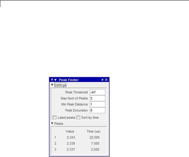
Peak Finder Panel
The Peak Finder panel displays maxima and the times at which they occur, allowing the settings for peak threshold, maximum number
of peaks, and peak excursion to be modified. You can choose to hide or display the Peak Finder panel. In the Scope menu, select
Tools > Measurements > Peak Finder. Alternatively, in the Scope toolbar, select the Peak Finder  button.
The Peak finder panel is separated into two panes, labeled Settings and Peaks. You can expand each pane to see the available options.
Settings Pane
The Settings pane enables you to modify the parameters used to calculate the peak values within the displayed portion of the input
2-1786

Time Scope
signal. For more information on the algorithms this pane uses, see the Signal Processing Toolbox findpeaks function reference.
•Peak Threshold — The level above which peaks are detected. This setting is equivalent to the MINPEAKHEIGHT parameter, which you can set when you run the findpeaks function.
•Max Num of Peaks — The maximum number of peaks to show. This setting is equivalent to the NPEAKS parameter, which you can set when you run the findpeaks function.
•Min Peaks Distance — The minimum number of samples between adjacent peaks. This setting is equivalent to the MINPEAKDISTANCE parameter, which you can set when you run the findpeaks function.
•Peak Excursion — The minimum height difference between a peak and its neighboring samples. Peak excursion is illustrated alongside peak threshold in the following figure.
Whereas the peak threshold is a minimum value necessary for a sample value to be a peak, the peak excursion is the minimum difference between a peak sample and the samples to its left and right
2-1787

Time Scope
in the time domain. In the figure, the green vertical line illustrates the lesser of the two height differences between the labeled peak and its neighboring samples. This height difference must be greater than the Peak Excursion value for the labeled peak to be classified as a peak. Compare this setting to peak threshold, which is illustrated by the red horizontal line. The amplitude must be above this horizontal line for the labeled peak to be classified as a peak.
The peak excursion setting is equivalent to the THRESHOLD parameter, which you can set when you run the findpeaks function.
•Label peaks — When this check box is selected, the Peak Finder displays the calculated peak values directly on the plot. By default, this check box is cleared and no values are displayed on the plot.
•Sort by time — When this check box is selected, the Peak Finder puts the largest calculated peak values in the time range shown in the display in time-sorted order. The Peak Finder displays the peak values in the Peaks pane. The Max Num of Peaks parameter still controls the number of peaks listed. By default, this check box is cleared and the Peak Finder panel displays the largest calculated peak values in the Peaks pane in decreasing order of peak height.
Peaks Pane
The Peaks pane displays all of the largest calculated peak values and the times at which the peaks occur, using the parameters you define in the Settings pane. You set the Max Num of Peaks parameter to specify the number of peaks shown in the list. Using the Sort by time check box, you set the order in which the peaks are listed.
The numerical values displayed in the Value column are equivalent to the pks output argument returned when you run the findpeaks function. The numerical values displayed in the Time column are similar to the locs output argument returned when you run the findpeaks function.
When you use the zoom options in the Scope, the peak locations automatically adjust to the time range shown in the display. In the Scope toolbar, click the Zoom In or Zoom X button to constrict the
2-1788
Time Scope
x-axis range of the display, and the statistics shown reflect this time range. For example, you can zoom in on one peak to make the Peak Finder panel display information about only that particular peak.
Properties |
The Properties dialog box controls various properties about the Time |
|
Dialog |
Scope displays. From the Time Scope menu, select View > Properties |
|
Box |
to open this dialog box. Alternatively, in the Time Scope toolbar, click |
|
|
the Properties |
button. |
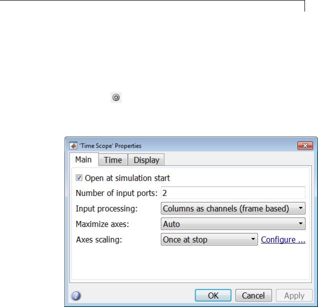
Main Pane
The Main pane of the Properties dialog box appears as follows.
2-1789

Time Scope
Open at simulation start
Select this check box to ensure that the Time Scope opens when the simulation starts.
Number of input ports
Specify the number of input ports that should appear on the left side of the Time Scope block.
Input processing
Specify whether the Time Scope should treat the input signal as
Columns as channels (frame based) or Elements as channels (sample based). Tunable.
Frame-based processing is only available for discrete input signals. For more information about frame-based input channels, see the “What
Is Frame-Based Processing?” section in the DSP System Toolbox documentation. For an example that uses the Time Scope block and frame-based input signals, see the Display Time-Domain Data in the Time Scope section in the DSP System Toolbox documentation.
Maximize axes
Specify whether to display the Time Scope in maximized axes mode. In this mode, each of the axes are expanded to fit into the entire display. To conserve space, no labels appear in each display. Instead, tick-mark values appear on top of the plotted data. You can select one of the following options:
•Auto — In this mode, the axes appear maximized in all displays only if the Title and Y-Axis label parameters are empty for every display. If you enter any value in any display for either of these parameters, the axes are not maximized.
•On — In this mode, the axes appear maximized in all displays. Any values entered into the Title and Y-Axis label parameters are hidden.
•Off — In this mode, none of the axes appear maximized.
The default setting is Auto.
2-1790

Time Scope
Axes scaling
Specify when the Time Scope should automatically scale the axes. You can select one of the following options:
•Manual — When you select this option, the Time Scope does not automatically scale the axes. You can manually scale the axes in any of the following ways:
-Select Tools > Scale axes limits.
-Press the Scale Axes Limits toolbar button.
-When the scope GUI is the active window, press Ctrl and A simultaneously.
•Auto — When you select this option, the Time Scope scales the axes as needed, both during and after simulation. Selecting this option enables the Do not allow Y-axis limits to shrink check box. By default, this parameter is selected, and the Time Scope does not shrink the y-axis limits when scaling the axes.
•Once at stop — Selecting this option causes the Time Scope to scale the axes each time simulation is stopped. The Time Scope does not scale the axes during simulation.
This parameter is Tunable.
Note Click the link labeled Configure to the right of the Axes scaling parameter to see additional axes scaling parameters. After you click this button, its label changes to Hide. To hide these additional parameters, click the Hide link.
Do not allow Y-axis limits to shrink
When you select this parameter, the y-axis limits are only allowed to grow during axes scaling operations. If you clear this check box, the y-axis limits may shrink during axes scaling operations.
2-1791

Time Scope
This parameter appears only when you select Auto for the Axis Scaling parameter. When you set the Axis Scaling parameter to Manual or Once at stop, the y-axis limits are allowed to shrink. Tunable.
Y-axis Data range (%)
Set the percentage of the y-axis the Scope should use to display the data when scaling the axes. Valid values are between 1 and 100. For example, if you set this parameter to 100, the Scope scales the y-axis limits such that your data uses the entire y-axis range. If you then set this parameter to 30, the Scope increases the y-axis range such that your data uses only 30% of the y-axis range. Tunable.
Y-axis Align
Specify where the Scope should align your data with respect to the y-axis when it scales the axes. You can select Top, Center, or Bottom. Tunable.
Scale X-axis limits
Check this box to allow the Scope to scale the x-axis limits when it scales the axes. Tunable.
X-axis Data range (%)
Set the percentage of the x-axis the Scope should use to display the data when scaling the axes. Valid values are between 1 and 100. For example, if you set this parameter to 100, the Scope scales the x-axis limits such that your data uses the entirex-axis range. If you then set this parameter to 30, the Scope increases the x-axis range such that your data uses only 30% of the x-axis range. Use the x-axis Align parameter to specify data placement with respect to the x-axis.
This parameter appears only when you select the Scale X-axis limits check box. Tunable.
X-axis Align
Specify how the Scope should align your data with respect to the x-axis: Left, Center, or Right. This parameter appears only when you select the Scale X-axis limits check box. Tunable.
Time Pane
The Time pane of the Properties dialog box appears as follows.
2-1792
Time Scope
Time span
Specify the time span, either by selecting a predefined option or by entering a numeric value in seconds. You can select one of the following options:
•Auto calculate — In this mode, the Time Scope automatically calculates the appropriate value for time span from the difference between the simulation “Start time” and “Stop time” parameters.
•One frame period — In this mode, the Time Scope uses the frame period of the input signal to the Time Scope block. This option is only available when the Input processing parameter is set to Columns as channels (frame based). This option is not available when you set the Input processing parameter to Elements as channels (sample based).
2-1793
Time Scope
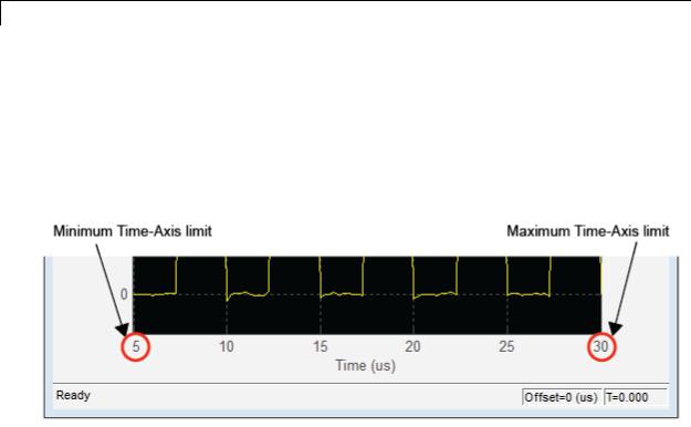
•<user defined> — In this mode, you specify the time span by replacing the text <user defined> with a numeric value in seconds.
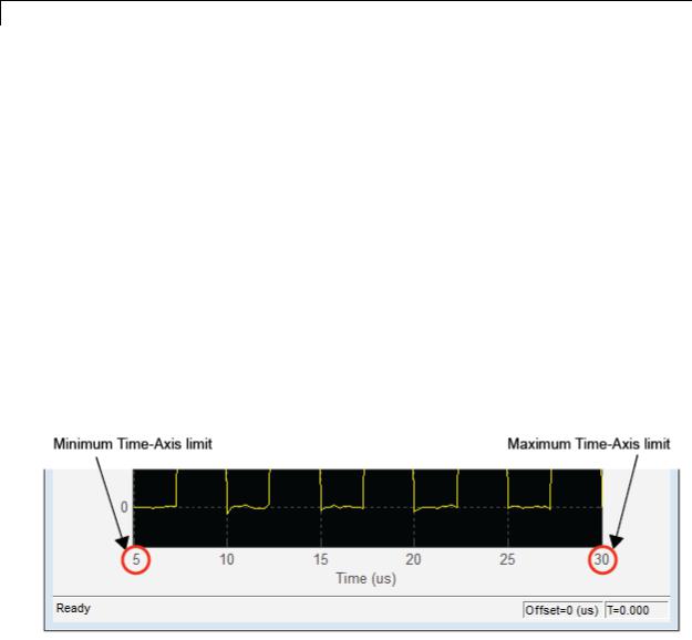
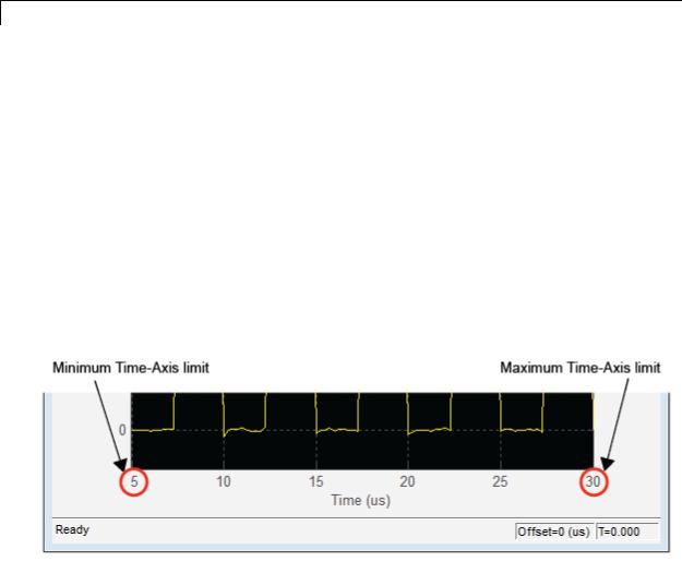
The scope sets the time-axis limits using the value of this parameter and the value of the Time display offset parameter. For example, if you set the Time display offset to 5e-6 and the Time span to 25e-6, the scope sets the time-axis limits as shown in the following figure.
Tunable. For more information, see “Signal Display” on page 2-1757.
Time span overrun
Specify how the scope displays new data beyond the visible time span. The default setting is Wrap. You can select one of the following options:
•Wrap — In this mode, the scope displays new data until the data reaches the maximum time-axis limit. When the data reaches the maximum time-axis limit of the scope window, the Time Scope clears the display. The Time Scope then updates the time offset value and begins displaying subsequent data points starting from the minimum time-axis limit.
•Scroll — In this mode, the scope scrolls old data to the left to make room for new data on the right side of the scope display. This mode is graphically intensive and can affect run-time performance, but it is beneficial for debugging and monitoring time-varying signals.
2-1794

Time Scope
This parameter is Tunable.
Time units
Specify the units used to describe the time-axis. The default setting is Metric. You can select one of the following options:
•Metric — In this mode, Time Scope converts the times on the time-axis to some metric units such as milliseconds, microseconds, nanoseconds, etc. Time Scope chooses the appropriate metric units, based on the minimum time-axis limit and the maximum time-axis limit of the scope window.
•Seconds — In this mode, Time Scope always displays the units on the time-axis as seconds.
•None — In this mode, Time Scope displays no units on the time-axis. Time Scope shows only the word Time on the time-axis.
Tunable.
Time display offset
This parameter allows you to offset the values displayed on the time-axis by a specified number of seconds. When you specify a scalar value, the scope offsets all channels equally. When you specify a vector of offset values, the scope offsets each channel independently. Tunable.
When you specify a Time display offset vector of length N, the scope offsets the input channels as follows:
•When N is equal to the number of input channels, the scope offsets each channel according to its corresponding value in the offset vector.
•When N is less than the number of input channels, the scope applies the values you specify in the offset vector to the first N input channels. The scope does not offset the remaining channels.
•When N is greater than the number of input channels, the scope offsets each input channel according to the corresponding value in the offset vector. The scope ignores all values in the offset vector that do not correspond to a channel of the input.
2-1795
Time Scope
The scope computes the time-axis range using the values of the Time display offset and Time span parameters. For example, if you set the
Time display offset to 5e-6 and the Time span to 25e-6, the scope sets the time-axis limits as shown in the following figure.
Similarly, when you specify a vector of values, the scope sets the minimum time-axis limit using the smallest value in the vector. To set the maximum time-axis limit, the scope sums the largest value in the vector with the value of the Time span parameter. For more information, see “Signal Display” on page 2-1757.
Show time-axis labels
Specify how to display the time units used to describe the time-axis. The default setting is All. You can select one of the following options:
•All — In this mode, the time-axis labels appear in all displays.
•None — In this mode, the time-axis labels do not appear in the displays.
•Bottom Displays Only — In this mode, the time-axis labels appear in only the bottom row of the displays.
Tunable.
2-1796
Time Scope
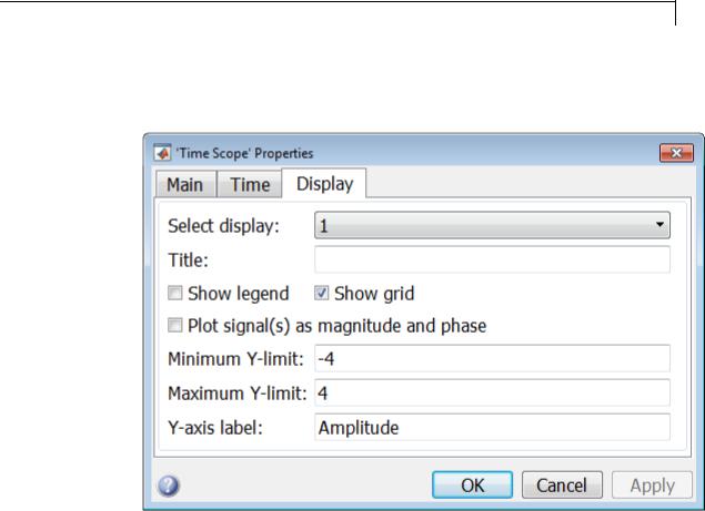
Display Pane
The Display pane of the Properties dialog box appears as follows.
Select Display
Specify the active display as a number, where a display number corresponds to the index of the input signal. The index of a display is its column-wise placement index. The default setting is 1. Set this parameter to control the display for which you intend to modify the title, legend, grid, y-axis limits, y-axis label, and magnitude/phase display parameters. Tunable.
Title
Specify the active display title as a string. By default, the active display has no title. Tunable.
2-1797

Time Scope
Show legend
Select this check box to show the legend in the active display. The channel legend displays a name for each channel of each input signal. When the legend appears, you can place it anywhere inside of the scope window. To turn the legend off, clear the Show legend check box. Tunable.
You can edit the name of any channel in the legend. To do so, double-click the current name, and enter a new channel name. By default, the scope names each channel according to either its signal name or the name of the block from which it comes. If the signal has multiple channels, the scope uses an index number to identify each channel of that signal. For example, a 2-channel signal named MySignal would have the following default names in the channel
legend: MySignal:1, MySignal:2.
The Time Scope does not display signal names that were labeled within an unmasked subsystem. You must label all input signals to the Time Scope block that originate from an unmasked subsystem.
To change the appearance of any channel of any input signal in the Time Scope window, from the Time Scope menu, select View > Style.
Show grid
When you select this check box, a grid appears in the active display of the Time Scope GUI. To hide the grid, clear this check box. Tunable.
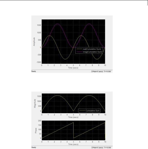
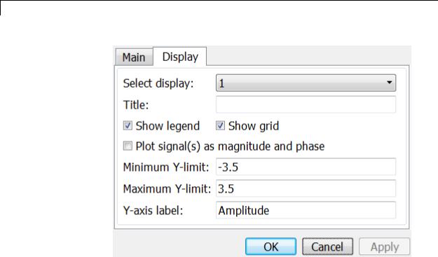
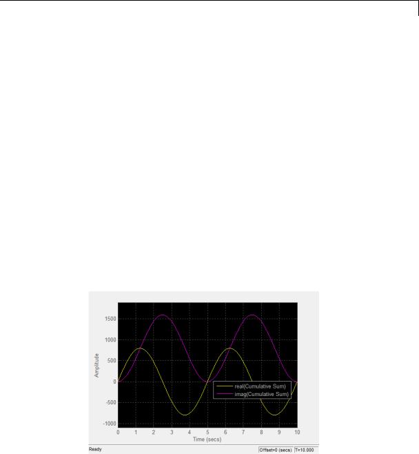
Plot signal(s) as magnitude and phase
When you select this check box, the Time Scope splits the magnitude and phase of the input signal on two separate axes within the same active display. By default, this box is cleared. If the input is a complex-valued signal, then the Time Scope plots the real and imaginary portions on the same display. These real and imaginary
portions appear as different-colored lines on the same axes within the same active display, as shown in the following figure.
2-1798
Time Scope
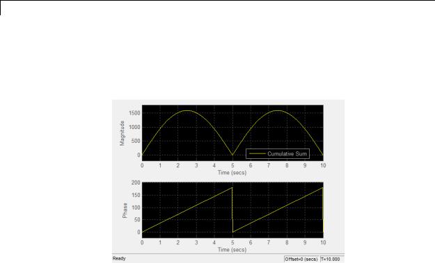
After you select this check box and click OK, the active display changes to show the magnitude of the input signal on the top axes and its phase, in degrees, on the bottom axes, as shown in the following figure.
This feature is particularly useful for complex-valued input signals. If the input is a real-valued signal, after you select this check box,
2-1799

Time Scope
|
the phase will be 0 degrees when the amplitude of the input signal |
|
is nonnegative and 180 degrees when the input signal is negative. |
|
Tunable. |
|
Minimum Y-limit |
|
Specify the minimum value of the y-axis. Tunable. |
|
When you select the Plot signal(s) as magnitude and phase check |
|
box, the value of this parameter always applies to the magnitude plot |
|
on the top axes. The phase plot on the bottom axes is always limited to |
|
a minimum value of –180 degrees. |
|
Maximum Y-limit |
|
Specify the maximum value of the y-axis. Tunable. |
|
When you select the Plot signal(s) as magnitude and phase check |
|
box, the value of this parameter always applies to the magnitude plot |
|
on the top axes. The phase plot on the bottom axes is always limited to |
|
a maximum value of 180 degrees. |
|
Y-axis label |
|
Specify the text for the scope to display to the left of the y-axis. Tunable. |
|
This parameter becomes invisible when you select the Plot signal(s) as |
|
magnitude and phase check box. When you enable that parameter, |
|
the y-axis label always appears as Magnitude on the top axes and Phase |
|
on the bottom axes. |
Style |
In the Style dialog box, you can customize the style of displays. You |
Dialog |
are able to change the color of the figure containing the displays, the |
Box |
background and foreground colors of display axes, and properties of |
|
lines in a display. From the Scope menu, select View > Style to open |
|
this dialog box. |
2-1800
Time Scope
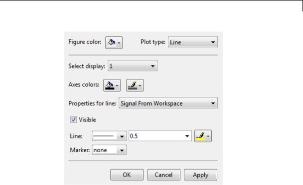
Properties
The Style dialog box allows you to modify the following properties of the Scope GUI:
Figure color
Specify the color that you want to apply to the background of the Scope GUI. By default, the figure color is gray.
Plot type
Specify the type of plot to use. The default setting is Line. Valid values for Plot type are:
•Line — Displays input signal as lines connecting each of the sampled values. This approach is similar to the functionality of the MATLAB line or plot function.
•Stairs — Displays input signal as a stairstep graph. A stairstep graph is made up of only horizontal lines and vertical lines. Each
2-1801

Time Scope
horizontal line represents the signal value for a discrete sample period and is connected to two vertical lines. Each vertical line represents a change in values occurring at a sample. This approach is equivalent to the MATLAB stairs function. Stairstep graphs are useful for drawing time history graphs of digitally sampled data.
•Auto — Displays input signal as a line graph if it is a continuous signal and displays input signal as a stairstep graph if it is a discrete signal.
This parameter is Tunable.
Select display
Specify the active display as a number, where a display number corresponds to the index of the input signal. The number of a display corresponds to its column-wise placement index. The default setting is 1. Set this parameter to control which display should have its axes colors, line properties, marker properties, and visibility changed. Tunable.
Axes colors
Specify the color that you want to apply to the background of the axes for the active display.
Properties for line
Specify the signal for which you want to modify the visibility, line properties, and marker properties.
Visible
Specify whether the selected signal on the active display should be visible. If you clear this check box, the line disappears.
Line
Specify the line style, line width, and line color for the selected signal on the active display.
Marker
Specify marks for the selected signal on the active display to show at data points. This parameter is similar to the Marker property for the MATLAB Handle Graphics® plot objects. You can choose any of the marker symbols from the following table.
2-1802
Time Scope
Simulation
Stepping
Options
|
Specifier |
Marker Type |
|
|
none |
No marker (default) |
|
|
|
Circle |
|
|
|
|
|
|
|
Square |
|
|
|
Cross |
|
|
|
Point |
|
|
|
Plus sign |
|
|
|
Asterisk |
|
|
|
Diamond |
|
|
|
Downward-pointing triangle |
|
|
|
Upward-pointing triangle |
|
|
|
Left-pointing triangle |
|
|
|
Right-pointing triangle |
|
|
|
Five-pointed star (pentagram) |
|
|
|
Six-pointed star (hexagram) |
|
|
|
|
|
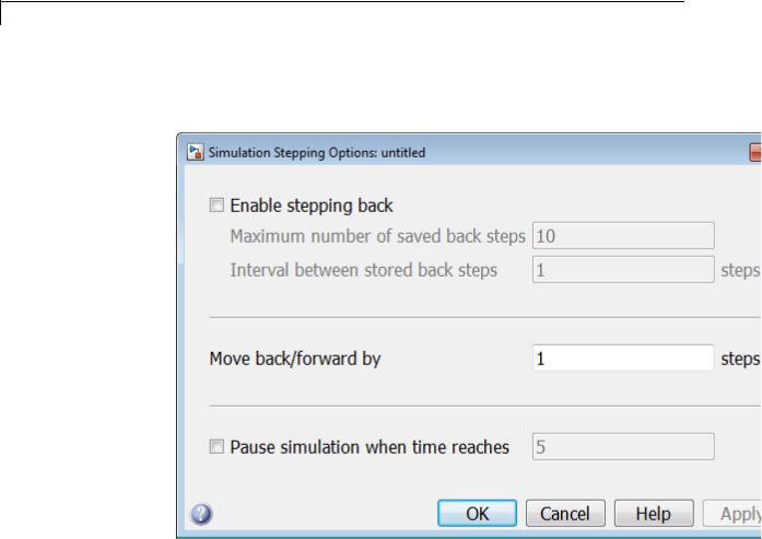
The Simulation Stepping Options dialog box lets you control the simulation behavior. You can pause the simulation at a specified time, enable stepping back, or specify options for stepping back.
You can also modify the number of steps by which to step forward or backward. To open this dialog box, in the Time Scope menu, select Simulation > Stepping Options to open this dialog box.
2-1803
Time Scope
Alternatively, if stepping back is disabled, in the Time Scope toolbar, click the previous step  button.
The Simulation Stepping Options dialog box is not unique to Time Scope; it can also be launched from any Simulink model. To open this dialog box from any Simulink model, select Simulation > Stepping Options. For more information, see “Simulation Stepping” in the Simulink documentation.
2-1804

Time Scope
Core —
General
UI Options
Enable stepping back
Select this check box to enable the Time Scope to take steps back in
time. When selected, Time Scope enables the previous step button ( ) on the simulation toolbar.
Maximum number of saved back steps
Specify the maximum number of back steps that the Time Scope saves in memory. To maximize simulation speed, the value for this parameter should be kept small. The default setting is 10.
Interval between stored back steps
Specify the number of steps between back steps that the Time Scope saves in memory for previous stepping. Set this parameter to a larger number to increase the time span of a back step without increasing the amount of memory used. The default setting is 1.
Move back/forward by
Specify the number of steps forward or backward that the Time Scope
progresses when you click the next step ( ) and previous step ( ) buttons. The default setting is 1.
Pause simulation when time reaches
Select this check box to enable the Time Scope to pause the simulation when it reaches a specified time.
Pause simulation when time reaches
Specify the time at which you want Time Scope to pause when the check box is selected.
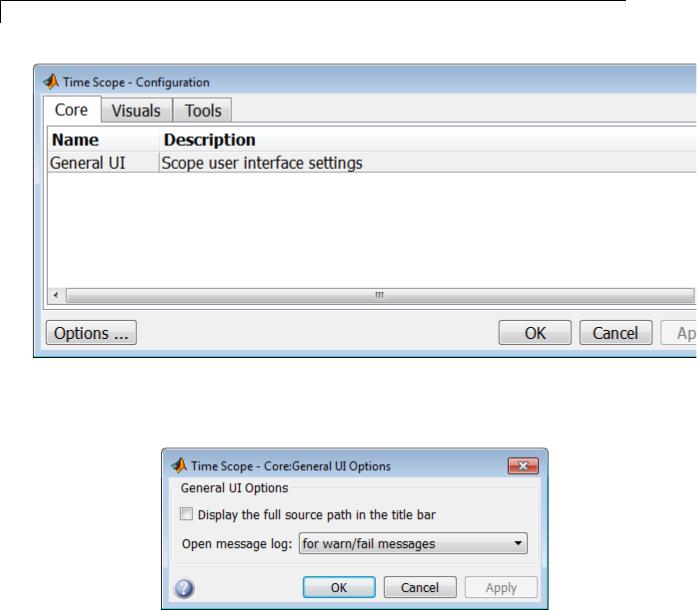
The Core:General UI Options dialog box controls the general settings for the Time Scope GUI. From the Time Scope menu bar, select
File > Configuration to open the Time Scope — Configuration dialog box. Click on the Core pane, and the following dialog box appears.
2-1805
Time Scope
To open the Core:General UI Options dialog box, select General UI and click Options. The following dialog box appears.
General UI Options
2-1806

Time Scope
Display the full source path in the title bar
If you select this check box, the Time Scope GUI displays the model name and full Simulink path to the data source in the title bar. Otherwise, a shortened name appears.
Open message log
Use this parameter to control when the Message Log window opens. The Message Log window helps you debug any issues with the Time Scope. Using the drop-down list, you can choose to open the Message Log window under any of the following conditions:
•for any new messages
•for warn/fail messages
•only for fail messages
•manually
You can open the Message Log at any time by selecting Help > Message Log. The Message Log dialog box provides a system-level record of loaded configuration settings and registered extensions. The Message Log displays summaries and details of each message, and you can filter the display of messages by Type and Category.
•The Type parameter allows you to select which types of messages to display in the Message Log. You can select All, Info, Warn, or Fail.
•The Category parameter allows you to select the category of messages to display in the Message Log. You can select All,
Configuration, or Extension.
-The scope uses Configuration messages to indicate when new configuration files are loaded.
-The scope uses Extension messages to indicate when components are registered. For example, you may see a Simulink registered message, indicating that a component has been successfully registered with Simulink and is available for configuration.
2-1807
Time Scope
Visuals
— Time
Domain
Options
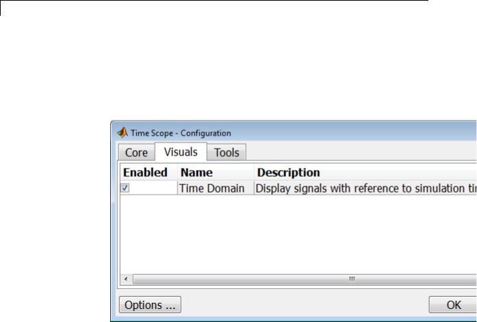
The Time Scope — Visuals:Time Domain Options dialog box controls the visual configuration settings of the Time Scope displays. You can open this dialog box from the Time Scope — Configuration dialog box. From the Time Scope menu bar, select File > Configuration to open the Time Scope — Configuration dialog box. Click the Visuals pane, and the following dialog box appears.
The Time Scope GUI has only one available visual, so you must ensure that the Enabled check box is selected. To open the Time Scope — Visuals:Time Domain Options dialog box, select Time Domain and click Options.
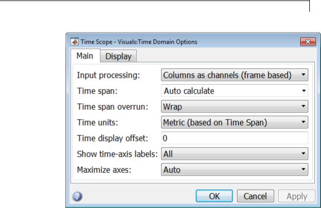
Main Pane
The Main pane of the Time Scope — Visuals:Time Domain Options dialog box appears as follows.
2-1808
Time Scope
Input processing
Specify whether the Time Scope should treat the input signal as
Columns as channels (frame based) or Elements as channels (sample based). Tunable.
Frame-based processing is only available for discrete input signals. For more information about frame-based input channels, see the “What Is Frame-Based Processing?” section in the DSP System Toolbox User’s Guide. For an example that uses the Time Scope block and frame-based input signals, see the Display Time-Domain Data in the Time Scope section in the DSP System Toolbox User’s Guide.
Time span
Specify the time span, either by selecting a predefined option or by entering a numeric value in seconds. You can select one of the following options:
2-1809
Time Scope
•Auto calculate — In this mode, the Time Scope automatically calculates the appropriate value for time span from the difference between the simulation “Start time” and “Stop time” parameters. This option is available only for the Time Scope block but not for the dsp.TimeScope System object.
•One frame period — In this mode, the Time Scope uses the frame period of the input signal to the Time Scope block. This option is only available when the Input processing parameter is set to Columns as channels (frame based). This option is not available when you set the Input processing parameter to Elements as channels (sample based).
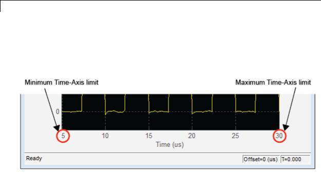
•<user defined> — In this mode, you specify the time span by replacing the text <user defined> with a numeric value in seconds.
The scope sets the time-axis limits using the value of this parameter and the value of the Time display offset parameter. For example, if you set the Time display offset to 5e-6 and the Time span to 25e-6, the scope sets the time-axis limits as shown in the following figure.
This parameter is Tunable.
Time span overrun
Specify how the scope displays new data beyond the visible time span. The default setting is Wrap. You can select one of the following options:
2-1810

Time Scope
•Wrap — In this mode, the scope displays new data until the data reaches the maximum time-axis limit. When the data reaches the maximum time-axis limit of the scope window, the Time Scope clears the display. The Time Scope then updates the time offset value, and begins displaying subsequent data points starting from the minimum time-axis limit.
•Scroll — In this mode, the scope scrolls old data to the left to make room for new data on the right side of the scope display. This mode is graphically intensive and can affect run-time performance, but it is beneficial for debugging and monitoring time-varying signals.
This parameter is Tunable.
Time units
Specify the units used to describe the time-axis. The default setting is Metric. You can select one of the following options:
•Metric — In this mode, Time Scope converts the times on the time-axis to some metric units such as milliseconds, microseconds, days, etc. Time Scope chooses the appropriate metric units, based on the minimum time-axis limit and the maximum time-axis limit of the scope window.
•Seconds — In this mode, Time Scope always displays the units on the time-axis as seconds.
•None — In this mode, Time Scope displays no units on the time-axis. Time Scope shows only the word Time on the time-axis.
This parameter is Tunable.
Time display offset
This parameter allows you to offset the values displayed on the time-axis by a specified number of seconds. When you specify a scalar value, the scope offsets all channels equally. When you specify a vector of offset values, the scope offsets each channel independently. Tunable.
When you specify a Time display offset vector of length N, the scope offsets the input channels as follows:
2-1811
Time Scope
•When N is equal to the number of input channels, the scope offsets each channel according to its corresponding value in the offset vector.
•When N is less than the number of input channels, the scope applies the values you specify in the offset vector to the first N input channels. The scope does not offset the remaining channels.
•When N is greater than the number of input channels, the scope offsets each input channel according to the corresponding value in the offset vector. The scope ignores all values in the offset vector that do not correspond to a channel of the input.
The scope computes the time-axis range using the values of the Time display offset and Time span parameters. For example, if you set the
Time display offset to 5e-6 and the Time span to 25e-6, the scope sets the time-axis limits as shown in the following figure.
Similarly, when you specify a vector of values, the scope sets the minimum time-axis limit using the smallest value in the vector. To set the maximum time-axis limit, the scope sums the largest value in the vector with the value of the Time span parameter. For more information, see “Signal Display” on page 2-1757.
Show time-axis labels
Specify how to display the time units used to describe the time-axis. The default setting is All. You can select one of the following options:
2-1812
Time Scope
•All — In this mode, the time-axis labels appear in all displays.
•None — In this mode, the time-axis labels do not appear in the displays.
•Bottom Displays Only — In this mode, the time-axis labels appear in only the bottom row of the displays.
Tunable.
Maximize axes
Specify whether to display the Time Scope in maximized axes mode. In this mode, each of the axes are expanded to fit into the entire display. In each display, there is no space to show labels. Tick mark values are shown on top of the plotted data. The default setting is Auto. You can select one of the following options:
•Auto — In this mode, the axes appear maximized in all displays only if the Title and Y-Axis label parameters are empty for every display. If you enter any value in any display for either of these parameters, the axes are not maximized.
•On — In this mode, the axes appear maximized in all displays. Any values entered into the Title and Y-Axis label parameters are hidden.
•Off — In this mode, none of the axes appear maximized.
Display Pane
The Display pane of the Visuals:Time Domain Options dialog box appears as follows.
2-1813
Time Scope
Select display
Specify the active display as a number, where a display number corresponds to the index of the input signal. The index of a display is its column-wise placement index. The default setting is 1. Set this parameter to control the display for which you intend to modify the title, legend, grid, y-axis limits, y-axis label, and magnitude/phase display parameters. Tunable.
Title
Specify the active display title as a string. By default, the active display has no title. Tunable.
Show legend
Select this check box to show the legend in the active display. The channel legend displays a name for each channel of each input signal. When the legend appears, you can place it anywhere inside of the scope window. To turn the legend off, clear the Show legend check box. Tunable.
2-1814
Time Scope
You can edit the name of any channel in the legend. To do so, double-click the current name, and enter a new channel name. By default, the scope names each channel according to either its signal name or the name of the block from which it comes. If the signal has multiple channels, the scope uses an index number to identify each channel of that signal. For example, a 2-channel signal named MySignal would have the following default names in the channel
legend: MySignal:1, MySignal:2.
To change the appearance of any channel of any input signal in the Scope window, from the menu, select View > Style.
Show grid
When you select this check box, a grid appears in the active display of the Scope. To hide the grid, clear this check box. Tunable.
Plot signal(s) as magnitude and phase
When you select this check box, the Scope splits the active display into a magnitude plot and a phase plot. By default, this check box is cleared. If the input signal is complex valued, the Scope plots the real and imaginary portions on the same axes. These real and imaginary portions appear as different-colored lines on the same axes within the same active display, as shown in the following figure.
2-1815
Time Scope
Selecting this check box and clicking the Apply or OK button changes the active display. The magnitude of the input signal appears on the top axes and its phase, in degrees, appears on the bottom axes. See the following figure.
This feature is particularly useful for complex-valued input signals. If the input is a real-valued signal, selecting this check box always produces the same behavior. The phase is 0 for nonnegative input and 180 degrees for negative input. Tunable.
Minimum Y-limit
Specify the minimum value of the y-axis. Tunable.
When you select the Plot signal(s) as magnitude and phase check box, the value of this parameter always applies to the magnitude plot on the top axes. The phase plot on the bottom axes is always limited to a minimum value of –180 degrees.
Maximum Y-limit
Specify the maximum value of the y-axis. Tunable.
When you select the Plot signal(s) as magnitude and phase check box, the value of this parameter always applies to the magnitude plot
2-1816

Time Scope
Tools —
Plot
Navigation
Options
on the top axes. The phase plot on the bottom axes is always limited to a maximum value of 180 degrees.
Y-axis label
Specify the text for the scope to display to the left of the y-axis. Tunable.
This parameter becomes invisible when you select the Plot signal(s) as magnitude and phase check box. When you enable that parameter, the y-axis label always appears as Magnitude on the top axes and Phase on the bottom axes.
The Tools:Plot Navigation Options dialog box provides you with the ability to automatically zoom in on and zoom out of your data, and to scale the axes of the Time Scope. In the Time Scope menu, select
Tools > Axes Scaling Options to open this dialog box.
Alternatively, you can open this dialog box from the Time Scope
— Configuration dialog box. In the Time Scope menu, select
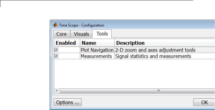
File > Configuration to open the Time Scope — Configuration dialog box. Click the Tools pane, and the following dialog box appears.
2-1817
Time Scope
The Tools pane in the Time Scope – Configuration dialog box contains the tools that appear on the Time Scope GUI. By default, the Plot Navigation tool is enabled. If you disable the tool by clearing the Enabled check box, the axes scaling and zoom tools no longer display in the Time Scope GUI. You can reenable the tool at any time by selecting the Enabled check box.
By default, the Measurements tool is also enabled. If you disable the tool by clearing the Enabled check box, the Time Domain Measurements tools no longer display in the Time Scope GUI. See the “Measurements Panels” on page 2-1766 section for more information. You can reenable the tool at any time by selecting the Enabled check box.
To open the Time Scope — Tools:Plot Navigation Options dialog box, select the Plot Navigation tool, and then click the Options button.
Parameters
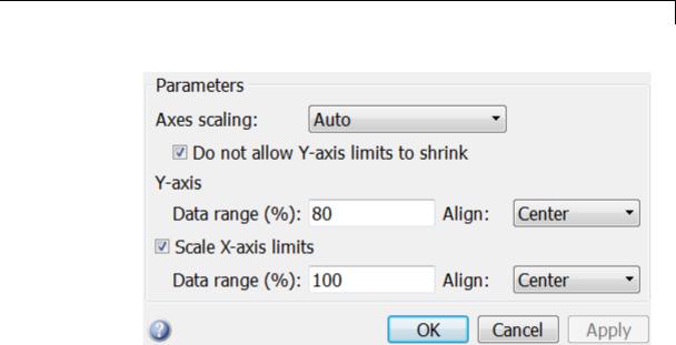
The Tools:Plot Navigation Options dialog box appears as follows.
2-1818
Time Scope
Axis Scaling
Specify when the Scope should automatically scale the axes. You can select one of the following options:
•Manual — When you select this option, the Scope does not automatically scale the axes. You can manually scale the axes in any of the following ways:
-Select Tools > Scale axes limits.
-Press the Scale Axes Limits toolbar button.
-When the scope GUI is the active window, press Ctrl+A.
•Auto — When you select this option, the Scope scales the axes as needed, both during and after simulation. Selecting this option enables the Do not allow Y-axis limits to shrink check box. By default, this parameter is selected, and the Scope does not shrink the y-axis limits when scaling the axes.
•Once at stop — Selecting this option causes the Scope to scale the axes each time simulation is stopped. The Scope does not scale the axes during simulation.
2-1819

Time Scope
This parameter is Tunable.
Do not allow Y-axis limits to shrink
When you select this parameter, the y-axis limits are only allowed to grow during axes scaling operations. If you clear this check box, the y-axis limits may shrink during axes scaling operations.
This parameter appears only when you select Auto for the Axis Scaling parameter. When you set the Axis Scaling parameter to Manual or Once at stop, the y-axis limits are allowed to shrink. Tunable.
Y-axis Data range (%)
Set the percentage of the y-axis that the Scope should use to display the data when scaling the axes. Valid values are between 1 and 100. For example, if you set this parameter to 100, the Scope scales the y-axis limits such that your data uses the entire y-axis range. If you then set this parameter to 30, the Scope increases the y-axis range such that your data uses only 30% of the y-axis range. Tunable.
Y-axis Align
Specify where the Scope should align your data with respect to the y-axis when it scales the axes. You can select Top, Center, or Bottom. Tunable.
Scale X-axis limits
Check this box to allow the Scope to scale the x-axis limits when it scales the axes. Tunable.
X-axis Data range (%)
Set the percentage of the x-axis that the Scope should use to display the data when scaling the axes. Valid values are between 1 and 100. For example, if you set this parameter to 100, the Scope scales the x-axis limits such that your data uses the entirex-axis range. If you then set this parameter to 30, the Scope increases the x-axis range such that your data uses only 30% of the x-axis range. Use the x-axis Align parameter to specify data placement with respect to the x-axis.
This parameter appears only when you select the Scale X-axis limits check box. Tunable.
2-1820
Time Scope
Sources —
Simulink
Options
Supported
Data
Types
X-axis Align
Specify how the Scope should align your data with respect to the x-axis: Left, Center, or Right. This parameter appears only when you select the Scale X-axis limits check box. Tunable.
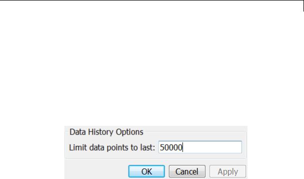
The Sources:Simulink Options dialog box lets you control the number of samples for each input signal that Time Scope holds in its memory cache. In the Time Scope menu, select View > Data History Options to open this dialog box.
Data History Options
Limit data points to last
Specify the number of data points for each input signal that Time Scope holds in its memory cache. The number of data points is equal to the product of the number of channels in the signal and the number of time samples. The default setting is 50000.
|
Port |
Supported Data Types |
|
|
Input |
• Double-precision floating point |
|
|
|
• Single-precision floating point |
|
|
|
• Fixed point (signed and unsigned) |
|
|
|
• Boolean |
|
|
|
• 8-, 16-, and 32-bit signed integers |
|
|
|
• 8-, 16-, and 32-bit unsigned integers |
|
|
|
• Simulink enumerations |
|
|
|
|
|
2-1821

Time Scope
Supported
Simulation
Modes
You can use the Time Scope block in models running the following supported simulation modes.
|
Mode |
SupportedNotes and Limitations |
|
|
|
Normal |
Yes |
|
|
|
Accelerator |
Yes |
|
|
|
Rapid |
Yes |
You can use Rapid Accelerator mode as a |
|
|
Accelerator |
|
method to increase the execution speed of |
|
|
|
|
your Simulink model. Rapid Accelerator |
|
|
|
|
mode creates an executable that includes the |
|
|
|
|
solver and model methods. This executable |
|
|
|
|
resides outside MATLAB and Simulink. |
|
|
|
|
Rapid Accelerator mode uses External |
|
|
|
|
mode to communicate with Simulink. For |
|
|
|
|
more information about Rapid Accelerator |
|
|
|
|
mode, see “Acceleration” in the Simulink |
|
|
|
|
documentation. |
|
|
PIL |
No |
|
|
|
SIL |
No |
|
|
|
External |
Yes |
You can use External mode to tune block |
|
|
|
|
parameters in real time and view block |
|
|
|
|
outputs in many types of blocks and |
|
|
|
|
subsystems. External mode establishes |
|
|
|
|
communication between a host system, |
|
|
|
|
where the Simulink environment resides, |
|
|
|
|
and a target system, where the executable |
|
|
|
|
runs after it is generated by the code |
|
|
|
|
generation and build process. For more |
|
|
|
|
information about External mode, see |
|
|
|
|
“Host/Target Communication” in the |
|
|
|
|
Simulink Coder documentation. |
|
|
|
|
Time Scope does not support data archiving. |
|
|
|
|
See “Set External Mode Data Archiving |
|
|
|
|
|
|
2-1822
Time Scope
Mode |
SupportedNotes and Limitations |
|
|
|
|
|
|
Parameters” in the Real-Time Windows |
|
|
Target™ documentation. |
|
|
Do not interactively open or close the Time |
|
|
Scope between the Connect and Start of the |
|
|
target. Attempting to do causes a checksum |
|
|
mismatch between the built model and the |
|
|
model in session. Open the Time Scope |
|
|
either before building or after starting the |
|
|
simulation. |
|
For more information about these modes, see “How Acceleration Modes |
|
Work” in the Simulink documentation. |
See Also |
Scope |
How To |
• “View Simulation Results” |
2-1823

To File
Purpose |
Write data to file |
Library Sinks
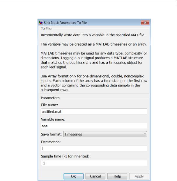
Description The To File block inputs a signal and writes the signal data to a MAT-file. Use the To File block to log signal data.
The To File block icon shows the name of the output file.
The block writes to the output file incrementally, with minimal memory overhead during simulation. If the output file exists when the simulation starts, the block overwrites the file. The file automatically closes when simulation is complete. If simulation terminates abnormally, the To File block saves the data it has logged up until the point of the abnormal termination.
Specifying the Format for Writing Data
Use the Save format parameter to specify which of the following two formats the To File block uses for writing data:
•Timeseries (default)
•Array
Use the Array format only for vector, double, noncomplex inputs. To save bus data, use the Timeseries format.
For the Timeseries format, the To File block:
•Writes data in a MATLAB timeseries object
•Supports writing multidimensional, real, or complex output values
•Supports writing output values that have any built-in data type, including Boolean, enumerated (enum), and fixed-point data with a word length of up to 32 bits
•For bus input signals, creates a MATLAB structure that matches the bus hierarchy. Each leaf of the structure is a MATLAB timeseries object.
2-1824

To File
For the Array format, the To File block:
•Writes data into a matrix containing two or more rows. The matrix has the following form:
|
t1 |
t2 |
|
tfinal |
|
|
u1 |
u1 |
u1 |
|
|
||
|
1 |
2 |
|
|
final |
|
|
|
|
|
|
|
|
|
|
un2 |
|
|
|
|
un1 |
unfinal |
|||||
|
|
|
|
|
|
|
Simulink writes one column to the matrix for each data sample. The first element of the column contains the time stamp. The remainder of the column contains data for the corresponding output values.
•Supports writing data that is one-dimensional, double, and noncomplex.
Controlling When Data Is Written to the File
The To File block Decimation and Sample Time parameters control when data is written to the file.
Saving Data for Use by a From File Block
The From File block can use data written by a To File block in any format (Timeseries or Array) without any modifications to the data or other special provisions.
Saving Data for Use by a From Workspace Block
The From Workspace block can read data that is in the Array format and is the transposition of the data written by the To File block. To provide the required format, use MATLAB commands to load and transpose the data from a MAT-file.
Simulation Stepper Interaction with To File Block
If you pause using the Simulation Stepper, the To File block captures the simulation data up to the point of the pause. When you step back,
2-1825

To File
Data Type
Support
the To File data file no longer contains any simulation data past the new reduced time of the last output.
Limitation on To File blocks in a Referenced Model
When a To File block is in a referenced model, that model must be a single-instance model. Only one instance of such a model can exist in a model hierarchy. See “General Reusability Limitations” for more information.
Compressing MAT-File Data
To avoid the overhead of compressing data in real time, the To File block writes an uncompressed Version 7.3 MAT-file. To compress the data within the MAT-file, load and save the file in MATLAB. The resaved file is smaller than the original MAT-file that the To File block created, because the Save command compresses the data in the MAT-file.
Saving Bus Data
The To File block supports virtual and nonvirtual bus input.
To save bus data, set the Save format parameter to Timeseries.
If the input signal is a bus, then the To File block creates a MATLAB structure that matches the bus hierarchy. Each leaf of the structure is a MATLAB timeseries object.
The To File block accepts real or complex signal data of any data type that Simulink supports, with the exception that the word length for fixed-point data must be 32 bits or less.
The To File block accepts bus data.
2-1826
To File
Parameters
2-1827

To File
and
Dialog |
File name |
|
Box |
The path or file name of the MAT-file in which to store the |
|
output. On UNIX systems, the pathname can start with a |
||
|
||
|
tilde (~) character signifying your home folder. The default file |
|
|
name is untitled.mat. If you specify a file name without path |
|
|
information, Simulink stores the file in the MATLAB working |
|
|
folder. (To determine the working folder, type pwd at the MATLAB |
|
|
command line.) If the file already exists, Simulink overwrites it. |
Variable name
The name of the matrix contained in the named file. The default name is ans.
Save format
The data format (timeseries or array) that the To File block uses for writing data. The default format is Timeseries.
Decimation
The decimation factor, n, where n specifies writing data at every nth time that the block executes. The default decimation is 1, which writes data at every time step.
Sample time
Specifies the sample period and offset at which to collect points. This parameter is useful when you are using a variable-step solver where the interval between time steps might not be constant. The default is-1, which inherits the sample time from the driving block. See “Specify Sample Time” for more information.
Characteristics |
|
Sample Time |
Specified in the Sample time |
|
|
|
parameter |
|
|
Dimensionalized |
Yes |
See Also |
|
“Export Runtime Information”, From File, From Workspace, To |
|
|
|
Workspace |
|
2-1828

To Workspace
Purpose |
Write data to MATLAB workspace |
Library Sinks
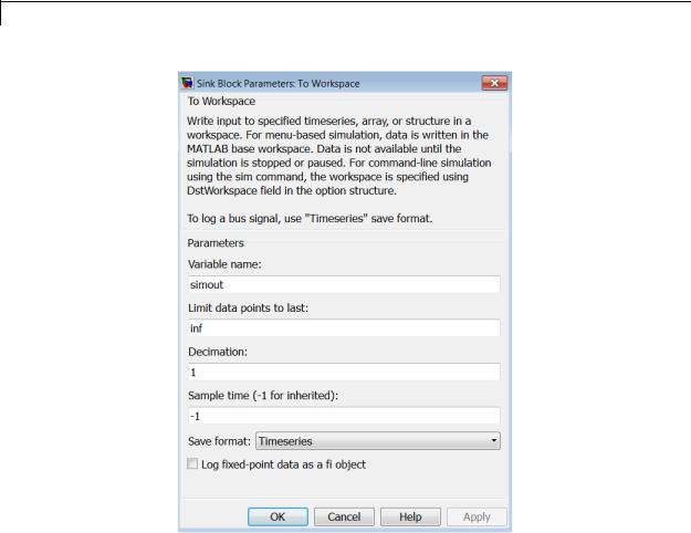
Description The To Workspace block inputs a signal and writes the signal data to the MATLAB workspace. During the simulation, the block writes data to an internal buffer. When the simulation is completed or paused, that data is written to the workspace. The block icon shows the name of the array to which the data is written.
To specify the name of the workspace variable to which the To Workspace block writes the data, use the Variable name parameter. To specify the data format of the variable, use the Save format parameter. You can specify to save the data in one of the following formats:
•A MATLAB timeseries object (or structure of MATLAB timeseries objects for bus data)
•An array
•Structure
•Structure with time
Saving Data for Use by a From Workspace Block
To use a From Workspace block to play back the sample-based data that was saved by a To Workspace block in a previous simulation, in the To Workspace block, use the Timeseries or Structure with time format.
Controlling the Amount of Data Saved
For variable-step solvers, to control the amount of data available to the To Workspace block, use the Model Configuration Parameters > Data Import/Export > Output options parameter. For example, have Simulink writes data at identical time points over multiple simulations, select the Produce specified output only option.
Then use To Workspace block parameters to control when and how much of this data the block writes:
2-1829

To Workspace
•Use the Limit data points to last parameter to specify how many sample points to save. If the simulation generates more data points than the specified maximum, the simulation saves only the most recently generated samples. To capture all the data, set this value to inf.
•Use the Decimation parameter to have the To Workspace block write data at every nth sample, where n is the decimation factor. The default decimation, 1, writes data at every time step.
•Use the Sample time parameter to specify a sampling interval at which to collect points. This parameter is useful when you are using a variable-step solver where the interval between time steps might not be the same. The default value of -1 causes the block to inherit the sample time from the driving block when determining the points to write. See “Specify Sample Time” in the online documentation for more information.
For example, suppose you have a simulation where the start time is 0, the Limit data points to last is 100, the Decimation is 1, and the
Sample time is 0.5. The To Workspace block collects a maximum of 100 points, at time values of 0, 0.5, 1.0, 1.5, ..., seconds. Specifying a Decimation value of 1 directs the block to write data at each step.
In a similar example, the Limit data points to last is 100 and the Sample time is 0.5, but the Decimation is 5. In this example, the block collects up to 100 points, at time values of 0, 2.5, 5.0, 7.5, ..., seconds. Specifying a Decimation value of 5 directs the block to write data at every fifth sample. The sample time ensures that data is written at these points.
In another example, all parameters are as defined in the first example except that the Limit data points to last is 3. In this case, only the last three sample points collected are written to the workspace. If the simulation stop time is 100, data corresponds to times 99.0, 99.5, and 100.0 seconds (three points).
2-1830

To Workspace
Data Type
Support
MAT-File Logging
If you enable the Model Configuration Parameters > Code Generation > Interface > MAT-file logging parameter, then To Workspace logs its data to a MAT-file.
The To Workspace block can save to the MATLAB workspace real or complex inputs of any data type that Simulink supports, including fixed-point and enumerated data types, as well as bus objects.
For more information, see “Data Types Supported by Simulink” in the Simulink documentation.
2-1831
To Workspace
Parameters |
|
|
and |
Variable name |
|
Dialog |
||
Specify the name of the variable to which to save the data. |
||
Box |
||
|
Limit data points to last |
|
|
Specify the maximum number of input samples to save. The default |
|
|
is inf. |
|
|
Decimation |
|
|
Specify the decimation factor. The default is 1. |
2-1832
To Workspace
Sample time
Specify the sample period and offset at which to collect data. This parameter is useful when you are using a variable-step solver where the interval between time steps might not be constant. The default is-1, which inherits the sample time from the driving block. See “Specify Sample Time” for more information.
Save format
Specify one of these formats for saving simulation output to the workspace:
•Timeseries — (Default)
Save non-bus signal input as a MATLAB timeseries object and bus signal input as a structure of MATLAB timeseries objects.
•Array
Save the input as an N-dimensional array where N is one more than the number of dimensions of the input signal. For example, if the input signal is a a vector, the resulting workspace array is two-dimensional. If the input signal is a matrix, then the array is three-dimensional.
How Simulink stores samples in the array depends on whether the input signal is a scalar or vector or a matrix. If the input is a scalar or a vector, each input sample is output as a row of the array. For example, suppose that the name of the output array is simout. Then, simout(1,:) corresponds to the first sample, simout(2,:) corresponds to the second sample, and so on. If the input signal is a matrix, the third dimension of the workspace array corresponds to the values of the input signal at specified sampling point. For example, suppose again that simout is the name of the resulting workspace array. Then, simout(:,:,1) is the value of the input signal at the first sample point; simout(:,:,2) is the value of the input signal at the second sample point; and so on.
•Structure
2-1833

To Workspace
This format consists of a structure with three fields:
-
-
-
time — This field is empty for this format.
signals — A structure with three fields: values, dimensions, and label. The values field contains the array of signal values. The dimensions field specifies the dimensions of the values array. The label field contains the label of the input line.
blockName — Name of the To Workspace block
•Structure With Time
This format is the same as Structure, except that the time field contains a vector of simulation time steps.
To read To Workspace block output directly with a From Workspace block, use either the Timeseries or Structure with Time format. For details, see “Techniques for Importing Signal Data”.
Structure with Time format does not support frame-based signals. Use Array or Structure format instead.
The support for simulation modes varies for the Timeseries format and non-Timeseries formats (Array, Structure, and Structure With Time).
|
Simulation |
Timeseries Format |
Non-Timeseries |
|
|
Mode |
|
Formats |
|
|
Normal |
Supported |
Supported |
|
|
|
|
|
|
|
Accelerator |
Supported for all |
Supported for models |
|
|
|
models, including |
without model |
|
|
|
model references |
references |
|
|
Rapid Accelerator |
Not supported |
Supported for models |
|
|
|
|
without model |
|
|
|
|
references |
|
2-1834

To Workspace
|
Simulation |
Timeseries Format |
Non-Timeseries |
|
|
Mode |
|
Formats |
|
|
External mode |
Not supported |
Supported for models |
|
|
|
|
without model |
|
|
|
|
references |
|
|
SIL and PIL |
Not supported |
Supported for models |
|
|
|
|
without model |
|
|
|
|
references |
|
|
Simulink Coder |
Not supported |
Supported for models |
|
|
Targets |
|
without model |
|
|
|
|
references |
|
Log fixed-point data as a fi object
Select to log fixed-point data to the MATLAB workspace as a Simulink Fixed-Point fi object. Otherwise, fixed-point data is logged to the workspace as double.
Examples |
The following example shows how to use the To Workspace block: |
||
|
|
• aero_vibrati |
|
Characteristics |
|
|
|
|
Sample Time |
Specified in the Sample time parameter |
|
|
|
Dimensionalized |
Yes |
|
|
Multidimensionalized |
Yes |
See Also |
|
“Data Export Basics”, From File, From Workspace, To File |
|
2-1835

Transfer Fcn
Purpose |
Model linear system by transfer function |
Library Continuous
Description The Transfer Fcn block models a linear system by a transfer function of the Laplace-domain variable s. The block can model single-input single-output (SISO) and single-input multiple output (SIMO) systems.
Conditions for Using This Block
The Transfer Fcn block assumes the following conditions:
• The transfer function has the form |
|
|
|
||||||
H(s) = |
y(s) |
= |
num(s) |
= |
num(1)snn−1 |
+ num(2)snn−2 |
+ + num(nn) |
, |
|
u(s) |
den(s) |
den(1)snd−1 + den(2)snd−2 |
+ + den(nd) |
||||||
|
|
|
|
||||||
where u and y are the system input and outputs, respectively, nn and nd are the number of numerator and denominator coefficients, respectively. num(s) and den(s) contain the coefficients of the numerator and denominator in descending powers of s.
•The order of the denominator must be greater than or equal to the order of the numerator.
•For a multiple-output system, all transfer functions have the same denominator and all numerators have the same order.
Modeling a Single-Output System
For a single-output system, the input and output of the block are scalar time-domain signals. To model this system:
1Enter a vector for the numerator coefficients of the transfer function in the Numerator coefficients field.
2Enter a vector for the denominator coefficients of the transfer function in the Denominator coefficients field.
2-1836

Transfer Fcn
Modeling a Multiple-Output System
For a multiple-output system, the block input is a scalar and the output is a vector, where each element is an output of the system. To model this system:
1Enter a matrix in the Numerator coefficients field.
Each row of this matrix contains the numerator coefficients of a transfer function that determines one of the block outputs.
2Enter a vector of the denominator coefficients common to all transfer functions of the system in the Denominator coefficients field.
Specifying Initial Conditions
Initial conditions are preset to zero. To specify initial conditions, convert to state-space form using tf2ss and use the State-Space block. The tf2ss utility provides the A, B, C, and D matrices for the system. For more information, type help tf2ss or see the Control System Toolbox™ documentation.
Transfer Function Display on the Block
The Transfer Fcn block displays the transfer function depending on how you specify the numerator and denominator parameters.
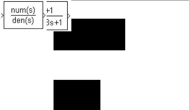
•If you specify each parameter as an expression or a vector, the block shows the transfer function with the specified coefficients and powers of s. If you specify a variable in parentheses, the block evaluates the variable.
For example, if you specify Numerator coefficients as [3,2,1] and Denominator coefficients as (den), where den is [7,5,3,1], the block looks like this:
2-1837
Transfer Fcn
Data Type
Support
•If you specify each parameter as a variable, the block shows the variable name followed by (s).
For example, if you specify Numerator coefficients as num and Denominator coefficients as den, the block looks like this:
The Transfer Fcn block accepts and outputs signals of type double.
For more information, see “Data Types Supported by Simulink” in the Simulink documentation.
2-1838
Transfer Fcn
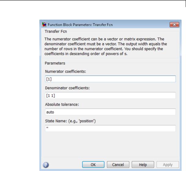
Parameters and Dialog Box
2-1839

Transfer Fcn
Numerator coefficients
Define the row vector of numerator coefficients.
Settings
Default: [1]
Tips
•For a single-output system, enter a vector for the numerator coefficients of the transfer function.
•For a multiple-output system, enter a matrix. Each row of this matrix contains the numerator coefficients of a transfer function that determines one of the block outputs.
Command-Line Information
See “Block-Specific Parameters” on page 8-109 for the command-line information.
2-1840

Transfer Fcn
Denominator coefficients
Define the row vector of denominator coefficients.
Settings
Default: [1 1]
Tips
•For a single-output system, enter a vector for the denominator coefficients of the transfer function.
•For a multiple-output system, enter a vector containing the denominator coefficients common to all transfer functions of the system.
Command-Line Information
See “Block-Specific Parameters” on page 8-109 for the command-line information.
2-1841

Transfer Fcn
Absolute tolerance
Specify the absolute tolerance for computing block states.
Settings
Default: auto
•You can enter auto, 1, a real scalar, or a real vector.
•If you enter auto or 1, then Simulink uses the absolute tolerance value in the Configuration Parameters dialog box (see “Solver Pane”) to compute block states.
•If you enter a real scalar, then that value overrides the absolute tolerance in the Configuration Parameters dialog box for computing all block states.
•If you enter a real vector, then the dimension of that vector must match the dimension of the continuous states in the block. These values override the absolute tolerance in the Configuration Parameters dialog box.
Command-Line Information
See “Block-Specific Parameters” on page 8-109 for the command-line information.
2-1842
Transfer Fcn
State Name (e.g., ’position’)
Assign a unique name to each state.
Settings
Default: ' '
If this field is blank, no name assignment occurs.
Examples
Tips
•To assign a name to a single state, enter the name between quotes, for example, 'velocity'.
•To assign names to multiple states, enter a comma-delimited list surrounded by braces, for example, {'a', 'b', 'c'}. Each name must be unique.
•The state names apply only to the selected block.
•The number of states must divide evenly among the number of state names.
•You can specify fewer names than states, but you cannot specify more names than states.
For example, you can specify two names in a system with four states. The first name applies to the first two states and the second name to the last two states.
•To assign state names with a variable in the MATLAB workspace, enter the variable without quotes. A variable can be a string, cell array, or structure.
Command-Line Information
See “Block-Specific Parameters” on page 8-109 for the command-line information.
The following Simulink examples show how to use the Transfer Fcn block:
• sldemo_f14
2-1843

Transfer Fcn
Characteristics
See Also
• sldemo_absbrake
• penddemo
Direct Feedthrough |
Only if the lengths of the Numerator |
|
coefficients and Denominator |
|
coefficients parameters are equal |
Sample Time |
Continuous |
Scalar Expansion |
No |
States |
Length of Denominator coefficients |
|
-1 |
Dimensionalized |
Yes, the block expands scalar input |
|
into vector output when the transfer |
|
function numerator is a matrix. |
Zero-Crossing Detection |
No |
|
|
Discrete Transfer Fcn
2-1844

Transfer Fcn Direct Form II
Purpose |
Implement Direct Form II realization of transfer function |
Library |
Additional Math & Discrete / Additional Discrete |
Description |
|
Data Type
Support
The Transfer Fcn Direct Form II block implements a Direct Form II realization of the transfer function that the Numerator coefficients and Denominator coefficients excluding lead parameters specify. The block supports only single input-single output (SISO) transfer functions.
The block automatically selects the data types and scalings of the output, the coefficients, and any temporary variables.
The Transfer Fcn Direct Form II block accepts signals of the following data types:
•Floating point
•Built-in integer
•Fixed point
For more information, see “Data Types Supported by Simulink” in the Simulink documentation.
2-1845
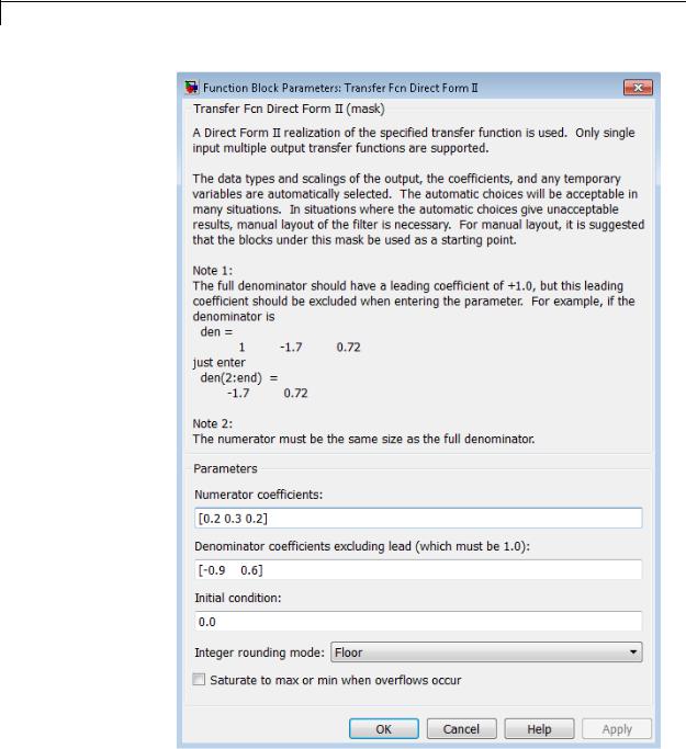
Transfer Fcn Direct Form II
Parameters and
Dialog |
Numerator coefficients |
Box |
Specify the numerator coefficients. |
2-1846 Denominator coefficients excluding lead
Specify the denominator coefficients, excluding the leading coefficient, which must be 1.0.

Transfer Fcn Direct Form II
Initial condition
Set the initial condition.
Integer rounding mode
Specify the rounding mode for fixed-point operations. For more information, see “Rounding”. in the Simulink Fixed Point documentation.
Saturate to max or min when overflows occur
Select to have overflows saturate to the maximum or minimum value that the data type can represent. Otherwise, overflows wrap.
When you select this check box, saturation applies to every internal operation on the block, not just the output or result. In general, the code generation process can detect when overflow is not possible. In this case, the code generator does not produce saturation code.
Characteristics
See Also
Direct Feedthrough |
Yes |
Scalar Expansion |
Yes, of initial conditions |
Multidimensionalized |
No |
Zero-Crossing Detection |
No |
|
|
Transfer Fcn Direct Form II Time Varying
2-1847

Transfer Fcn Direct Form II Time Varying
Purpose |
Implement time varying Direct Form II realization of transfer function |
Library |
Additional Math & Discrete / Additional Discrete |
Description |
|
Data Type
Support
The Transfer Fcn Direct Form II Time Varying block implements a Direct Form II realization of the specified transfer function. The block supports only single input-single output (SISO) transfer functions.
The input signal labeled Den No Lead contains the denominator coefficients of the transfer function. The full denominator has a leading coefficient of one, but it is excluded from the input signal. For example, a denominator of [1 -1.7 0.72] is represented by a signal with the value [-1.7 0.72]. The input signal labeled Num contains the numerator coefficients. The data types of the numerator and denominator coefficients can be different, but the length of the numerator vector and the full denominator vector must be the same. Pad the numerator vector with zeros, if needed.
The block automatically selects the data types and scalings of the output, the coefficients, and any temporary variables.
The Transfer Fcn Direct Form II Time Varying block accepts signals of the following data types:
•Floating point
•Built-in integer
•Fixed point
2-1848

Transfer Fcn Direct Form II Time Varying
For more information, see “Data Types Supported by Simulink” in the Simulink documentation.
2-1849
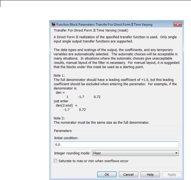
Transfer Fcn Direct Form II Time Varying
Parameters and
Dialog |
Initial condition |
Box |
Set the initial condition. |
|
2-1850

Transfer Fcn Direct Form II Time Varying
Integer rounding mode
Specify the rounding mode for fixed-point operations. For more information, see “Rounding”. in the Simulink Fixed Point documentation.
Saturate to max or min when overflows occur
Select to have overflows saturate to the maximum or minimum value that the data type can represent. Otherwise, overflows wrap.
When you select this check box, saturation applies to every internal operation on the block, not just the output or result. In general, the code generation process can detect when overflow is not possible. In this case, the code generator does not produce saturation code.
Characteristics
See Also
Direct Feedthrough |
Yes |
Scalar Expansion |
Yes, of initial conditions |
Multidimensionalized |
No |
Zero-Crossing Detection |
No |
|
|
Transfer Fcn Direct Form II
2-1851
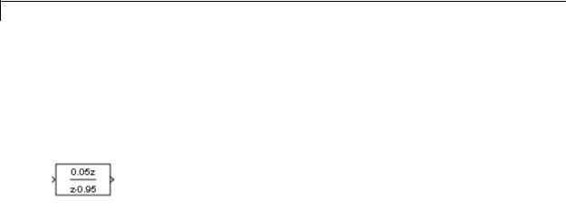
Transfer Fcn First Order
Purpose |
Implement discrete-time first order transfer function |
Library Discrete
Description The Transfer Fcn First Order block implements a discrete-time first order transfer function of the input. The transfer function has a unity DC gain.
Data Type |
The Transfer Fcn First Order block accepts signals of the following |
Support |
data types: |
|
• Floating point |
|
• Built-in integer |
|
• Fixed point |
|
For more information, see “Data Types Supported by Simulink” in the |
|
Simulink documentation. |
2-1852
Transfer Fcn First Order
Parameters and Dialog Box
Pole (in Z plane)
Set the pole.
Initial condition for previous output
Set the initial condition for the previous output.
Integer rounding mode
Specify the rounding mode for fixed-point operations. For more information, see “Rounding”. in the Simulink Fixed Point documentation.
Saturate to max or min when overflows occur
Select to have overflows saturate to the maximum or minimum value that the data type can represent. Otherwise, overflows wrap.
2-1853

Transfer Fcn First Order
When you select this check box, saturation applies to every internal operation on the block, not just the output or result. In general, the code generation process can detect when overflow is not possible. In this case, the code generator does not produce saturation code.
Characteristics |
Direct Feedthrough |
Yes |
|
Scalar Expansion |
Yes, of initial conditions |
|
Zero-Crossing Detection |
No |
|
|
|
2-1854

Transfer Fcn Lead or Lag
Purpose |
Implement discrete-time lead or lag compensator |
Library |
Discrete |
Description |
The Transfer Fcn Lead or Lag block implements a discrete-time |
|
lead or lag compensator of the input. The instantaneous gain of the |
|
compensator is one, and the DC gain is equal to (1-z)/(1-p), where z is |
|
the zero and p is the pole of the compensator. |
|
The block implements a lead compensator when 0 < z < p < 1, and |
|
implements a lag compensator when 0 < p < z < 1. |
Data Type |
The Transfer Fcn Lead or Lag block accepts signals of any numeric data |
Support |
type that Simulink supports, including fixed-point data types. |
|
For more information, see “Data Types Supported by Simulink” in the |
|
Simulink documentation. |
2-1855
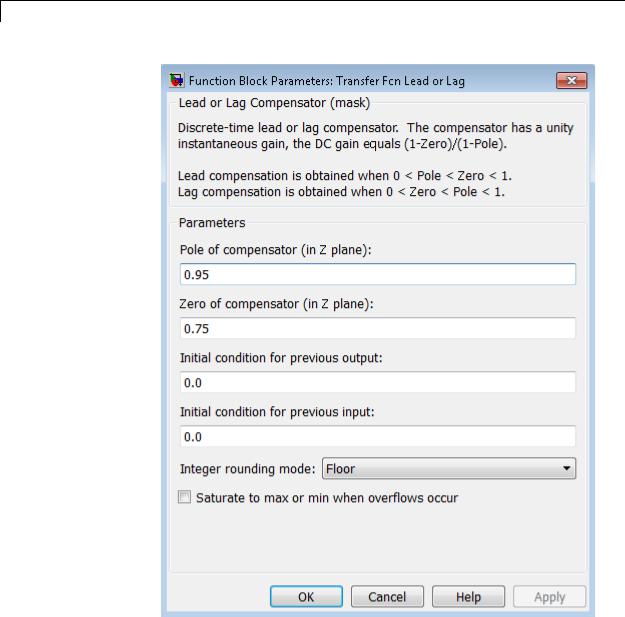
Transfer Fcn Lead or Lag
Parameters
2-1856

Transfer Fcn Lead or Lag
and
Dialog |
Pole of compensator (in Z plane) |
||
Box |
Set the pole. |
|
|
Zero of compensator (in Z plane) |
|||
|
|||
|
Set the zero. |
|
|
|
Initial condition for previous output |
||
|
Set the initial condition for the previous output. |
||
|
Initial condition for previous input |
||
|
Set the initial condition for the previous input. |
||
|
Integer rounding mode |
|
|
|
Specify the rounding mode for fixed-point operations. For more |
||
|
information, see “Rounding”. in the Simulink Fixed Point |
||
|
documentation. |
|
|
|
Saturate to max or min when overflows occur |
||
|
Select to have overflows saturate to the maximum or minimum |
||
|
value that the data type can represent. Otherwise, overflows |
||
|
wrap. |
|
|
|
When you select this check box, saturation applies to every |
||
|
internal operation on the block, not just the output or result. In |
||
|
general, the code generation process can detect when overflow is |
||
|
not possible. In this case, the code generator does not produce |
||
|
saturation code. |
|
|
Characteristics |
|
|
|
Direct Feedthrough |
Yes |
||
|
Scalar Expansion |
Yes, of initial conditions |
|
|
Zero-Crossing Detection |
No |
|
|
|
|
|
2-1857

Transfer Fcn Real Zero
Purpose |
Implement discrete-time transfer function that has real zero and no pole |
Library Discrete
Description The Transfer Fcn Real Zero block implements a discrete-time transfer function that has a real zero and effectively no pole.
Data Type |
The Transfer Fcn Real Zero block accepts signals of any numeric data |
Support |
type that Simulink supports, including fixed-point data types. |
|
For more information, see “Data Types Supported by Simulink” in the |
|
Simulink documentation. |
2-1858
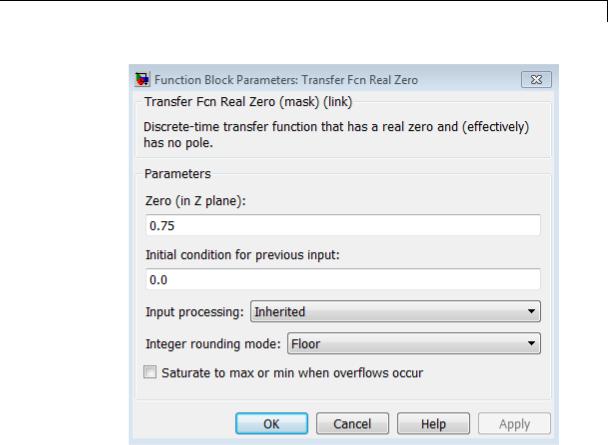
Transfer Fcn Real Zero
Parameters and Dialog Box
Zero (in Z plane)
Set the zero.
Initial condition for previous input
Set the initial condition for the previous input.
Input processing
Specify whether the block performs sampleor frame-based processing. You can select one of the following options:
•Elements as channels (sample based) — Treat each element of the input as a separate channel (sample-based processing).
2-1859

Transfer Fcn Real Zero
•Columns as channels (frame based) — Treat each column of the input as a separate channel (frame-based processing).
Note Frame-based processing requires a DSP System Toolbox license.
For more information, see “Sampleand Frame-Based Concepts” in the DSP System Toolbox documentation.
•Inherited — Inherit the processing mode from the input signal and delay the input accordingly. You can identify whether the input signal is sample or frame based by looking at the signal line. Simulink represents sample-based signals with a single line and frame-based signals with a double line.
Note When you choose the Inherited option for the Input processing parameter, and the input signal is frame-based, Simulink® will generate a warning or error in future releases.
Use Input processing to specify whether the block performs sampleor frame-based processing. The block accepts frame-based signals for the input u. All other input signals must be sample based.
|
Input Signal u |
Input Processing |
Block Works? |
|
|
|
Mode |
|
|
|
Sample based |
Sample based |
Yes |
|
|
Frame based |
|
No, produces an |
|
|
|
|
error |
|
|
Sample based |
Frame based |
Yes |
|
|
Frame based |
|
Yes |
|
|
|
|
|
|
2-1860

Transfer Fcn Real Zero
|
Input Signal u |
Input Processing |
Block Works? |
|
|
|
Mode |
|
|
|
Sample based |
Inherited |
Yes |
|
|
Frame based |
|
Yes |
|
|
|
|
|
|
For more information about these two processing modes, see “Sampleand Frame-Based Concepts” in the DSP System Toolbox documentation.
Integer rounding mode
Specify the rounding mode for fixed-point operations. For more information, see “Rounding”. in the Simulink Fixed Point documentation.
Saturate to max or min when overflows occur
Select to have overflows saturate to the maximum or minimum value that the data type can represent. Otherwise, overflows wrap.
When you select this check box, saturation applies to every internal operation on the block, not just the output or result. In general, the code generation process can detect when overflow is not possible. In this case, the code generator does not produce saturation code.
Characteristics |
Direct Feedthrough |
Yes |
|
Scalar Expansion |
Yes, of initial conditions |
|
Zero-Crossing Detection |
No |
|
|
|
2-1861

Transport Delay
Purpose |
Delay input by given amount of time |
Library Continuous
Description The Transport Delay block delays the input by a specified amount of time. You can use this block to simulate a time delay. The input to this block should be a continuous signal.
At the start of simulation, the block outputs the Initial output parameter until the simulation time exceeds the Time delay parameter. Then, the block begins generating the delayed input. During simulation, the block stores input points and simulation times in a buffer. You specify this size with the Initial buffer size parameter.
When you want output at a time that does not correspond to times of the stored input values, the block interpolates linearly between points. When the delay is smaller than the step size, the block extrapolates from the last output point, which can produce inaccurate results. Because the block does not have direct feedthrough, it cannot use the current input to calculate an output value. For example, consider a fixed-step simulation with a step size of 1 and the current time at t = 5. If the delay is 0.5, the block must generate a point at t = 4.5. Because the most recent stored time value is at t = 4, the block performs forward extrapolation.
The Transport Delay block does not interpolate discrete signals. Instead, the block returns the discrete value at the required time.
This block differs from the Unit Delay block, which delays and holds the output on sample hits only.
Tip Avoid using linmod to linearize a model that contains a Transport Delay block. For more information, see “Linearizing Models” in the Simulink documentation.
2-1862
Transport Delay
Data Type
Support
The Transport Delay block accepts and outputs real signals of type double.
For more information, see “Data Types Supported by Simulink” in the Simulink documentation.
2-1863
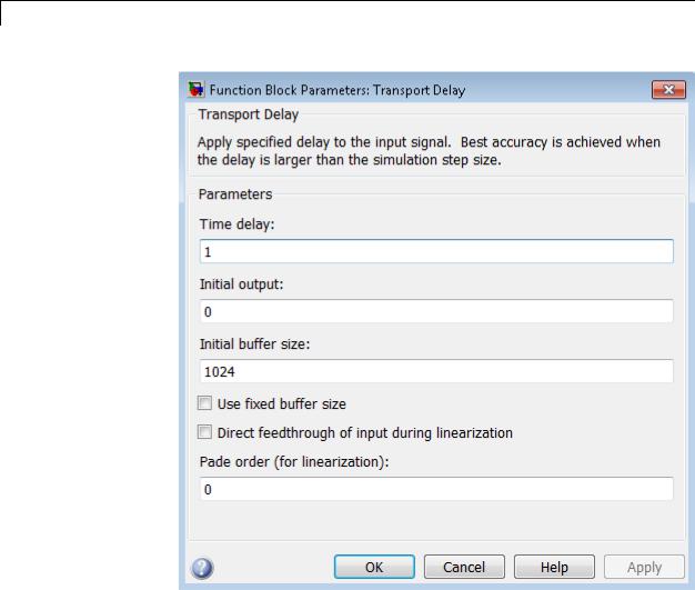
Transport Delay
Parameters and Dialog Box
2-1864

Transport Delay
Time delay
Specify the amount of simulation time to delay the input signal before propagation to the output.
Settings
Default: 1
This value must be nonnegative.
Command-Line Information
See “Block-Specific Parameters” on page 8-109 for the command-line information.
2-1865

Transport Delay
Initial output
Specify the output that the block generates until the simulation time first exceeds the time delay input.
Settings
Default: 0
The initial output of this block cannot be inf or NaN.
Command-Line Information
See “Block-Specific Parameters” on page 8-109 for the command-line information.
2-1866

Transport Delay
Initial buffer size
Define the initial memory allocation for the number of input points to store.
Settings
Default: 1024
•If the number of input points exceeds the initial buffer size, the block allocates additional memory.
•After simulation ends, a message shows the total buffer size needed.
Tips
•Because allocating memory slows down simulation, choose this value carefully if simulation speed is an issue.
•For long time delays, this block can use a large amount of memory, particularly for dimensionalized input.
Command-Line Information
See “Block-Specific Parameters” on page 8-109 for the command-line information.
2-1867

Transport Delay
Use fixed buffer size
Specify use of a fixed-size buffer to save input data from previous time steps.
Settings
Default: Off
 On
On
The block uses a fixed-size buffer.
 Off
Off
The block does not use a fixed-size buffer.
The Initial buffer size parameter specifies the size of the buffer. If the buffer is full, new data replaces data already in the buffer. Simulink software uses linear extrapolation to estimate output values that are not in the buffer.
Note If you have a Simulink Coder license, ERT or GRT code generation uses a fixed-size buffer even if you do not select this check box.
Tips
•If the input data is linear, selecting this check box can save memory.
•If the input data is nonlinear, do not select this check box. Doing so can yield inaccurate results.
Command-Line Information
See “Block-Specific Parameters” on page 8-109 for the command-line information.
2-1868

Transport Delay
Direct feedthrough of input during linearization
Cause the block to output its input during linearization and trim, which sets the block mode to direct feedthrough.
Settings
Default: Off
 On
On
Enables direct feedthrough of input.
 Off
Off
Disables direct feedthrough of input.
Tips
•Selecting this check box can cause a change in the ordering of states in the model when you use the functions linmod, dlinmod, or trim. To extract this new state ordering:
1Compile the model using the following command, where model is the name of the Simulink model.
[sizes, x0, x_str] = model([],[],[],'lincompile');
2 Terminate the compilation with the following command.
model([],[],[],'term');
•The output argument x_str, which is a cell array of the states in the Simulink model, contains the new state ordering. When you pass a vector of states as input to the linmod, dlinmod, or trim functions, the state vector must use this new state ordering.
Command-Line Information
See “Block-Specific Parameters” on page 8-109 for the command-line information.
2-1869

Transport Delay
Pade order (for linearization)
Set the order of the Pade approximation for linearization routines.
Settings
Default: 0
•The default value is 0, which results in a unity gain with no dynamic states.
•Setting the order to a positive integer n adds n states to your model, but results in a more accurate linear model of the transport delay.
Command-Line Information
See “Block-Specific Parameters” on page 8-109 for the command-line information.
Characteristics |
|
Direct Feedthrough |
No |
|
|
Sample Time |
Continuous |
|
|
Scalar Expansion |
Yes, of input and all parameters except |
|
|
|
Initial buffer size |
|
|
Dimensionalized |
Yes |
|
|
Zero-Crossing Detection |
No |
See Also |
|
Variable Time Delay |
|
2-1870

Trigger
Purpose
Library
Description
Data Type
Support
Add trigger port to model or subsystem
Ports & Subsystems
Adding a Trigger block to a model allows an external signal to trigger its execution. You can add a trigger port to a root-level model or to a subsystem.
Configure the Trigger block to execute the model either:
•Once on each integration step, when the value of the external signal changes in a way that you specify.
•Multiple times during a time step, when the external signal is a function-call from a Function-Call Generator block or S-function.
Include only one Trigger block in a model or a subsystem.
Specify the properties that the trigger port enforces for any incoming signal, using the Signal Attributes tab.
The Trigger block supports signal label propagation. For more information, see:
•“Triggered Subsystems”
•“Create Conditional Models”
•“Function-Call Models”
•“Function-Call Subsystems”
The Trigger block accepts signals of supported Simulink numeric data types, including fixed-point data types. For more information, see “Data Types Supported by Simulink” in the Simulink documentation.
2-1871
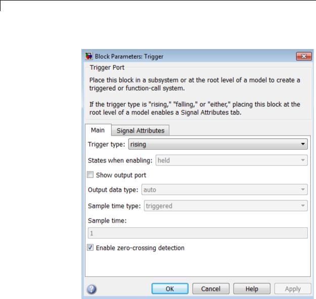
Trigger
Parameters The Main tab of the Trigger block dialog box appears as follows:
and Dialog Box
The Signal Attributes tab of the Trigger block dialog box appears as follows:
2-1872
Trigger
•“Trigger type” on page 2-1875
•“States when enabling” on page 2-1876
•“Propagate sizes of variable-size signals” on page 2-1878
2-1873

Trigger
•“Show output port” on page 2-1879
•“Output data type” on page 2-1880
•“Sample time type” on page 2-1881
•“Sample time” on page 2-1882
•“Enable zero-crossing detection” on page 2-1883
•“Port dimensions” on page 2-1884
•“Trigger signal sample time” on page 2-1885
•“Minimum” on page 2-1886
•“Maximum” on page 2-1887
•“Data type” on page 2-1888
•“Mode” on page 2-1890
•“Data type override” on page 2-1892
•“Signedness” on page 2-1893
•“Scaling” on page 2-1894
•“Word length” on page 2-1896
•“Fraction length” on page 2-1897
•“Slope” on page 2-1898
•“Bias” on page 2-1898
•“Interpolate data” on page 2-1899
2-1874