

Chapter 13: Creating Formulas That Count and Sum
Getting a Quick Count or Sum
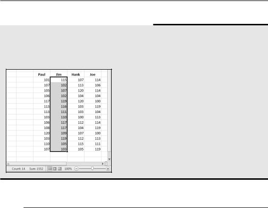
The Excel status bar can display useful information about the currently selected cells — no formulas required. Normally, the status bar displays the sum and count of the values in the selected range. You can, however, right-click to bring up a menu with other options. You can choose any or all the following: Average, Count, Numerical Count, Minimum, Maximum, and Sum.
Basic Counting Formulas
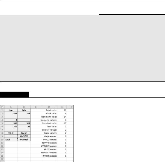
The basic counting formulas presented in this section are all straightforward and relatively simple. They demonstrate the capability of the Excel counting functions to count the number of cells in a range that meet specific criteria. Figure 13.1 shows a worksheet that uses formulas (in column E) to summarize the contents of range A1:B10 — a 20-cell range named Data. This range contains a variety of information, including values, text, logical values, errors, and empty cells.
On the CD
This workbook is available on the companion CD-ROM. The file is named basic counting.xlsx.
Counting the total number of cells
To get a count of the total number of cells in a range (empty and non-empty cells), use the following formula. This formula returns the number of cells in a range named Data. It simply multiplies the number of rows (returned by the ROWS function) by the number of columns (returned by the COLUMNS function).
=ROWS(Data)*COLUMNS(Data)
This formula will not work if the Data range consists of noncontiguous cells. In other words, Data must be a rectangular range of cells.
283
Part II: Working with Formulas and Functions
About This Chapter’s Examples
Most of the examples in this chapter use named ranges for function arguments. When you adapt these formulas for your own use, you’ll need to substitute either the actual range address or a range name defined in your workbook.
Also, some examples consist of array formulas. An array formula is a special type of formula that enables you to perform calculations that would not otherwise be possible. You can spot an array formula because it’s enclosed in curly brackets when it’s displayed in the Formula bar. In addition, I use this syntax for the array formula examples presented in this book. For example:
{=Data*2}
When you enter an array formula, press Ctrl+Shift+Enter (not just Enter) but don’t type the curly brackets (Excel inserts the brackets for you.) If you need to edit an array formula, don’t forget to use Ctrl+Shift+Enter when you finish editing (otherwise, the array formula will revert to a normal formula, and it will return an incorrect result). See Chapter 16 for an introduction to array formulas.
FIGURE 13.1
Formulas in column E display various counts of the data in A1:B10.
Counting blank cells
The following formula returns the number of blank (empty) cells in a range named Data:
=COUNTBLANK(Data)
The COUNTBLANK function also counts cells containing a formula that returns an empty string. For example, the formula that follows returns an empty string if the value in cell A1 is greater than 5. If the cell meets this condition, the COUNTBLANK function counts that cell.
=IF(A1>5,””,A1)
284
Chapter 13: Creating Formulas That Count and Sum
You can use the COUNTBLANK function with an argument that consists of entire rows or columns. For example, this next formula returns the number of blank cells in column A:
=COUNTBLANK(A:A)
The following formula returns the number of empty cells on the entire worksheet named Sheet1. You must enter this formula on a sheet other than Sheet1, or it will create a circular reference.
=COUNTBLANK(Sheet1!1:1048576)
Counting nonblank cells
To count nonblank cells, use the COUNTA function. The following formula uses the COUNTA function to return the number of nonblank cells in a range named Data:
=COUNTA(Data)
The COUNTA function counts cells that contain values, text, or logical values (TRUE or FALSE).
Note
If a cell contains a formula that returns an empty string, that cell is included in the count returned by COUNTA, even though the cell appears to be blank. n
Counting numeric cells
To count only the numeric cells in a range, use the following formula (which assumes the range is named Data):
=COUNT(Data)
Cells that contain a date or a time are considered to be numeric cells. Cells that contain a logical value (TRUE or FALSE) aren’t considered to be numeric cells.
Counting text cells
To count the number of text cells in a range, you need to use an array formula. The array formula that follows returns the number of text cells in a range named Data:
{=SUM(IF(ISTEXT(Data),1))}
Counting nontext cells
The following array formula uses the Excel ISNONTEXT function, which returns TRUE if its argument refers to any nontext cell (including a blank cell). This formula returns the count of the number of cells not containing text (including blank cells):
{=SUM(IF(ISNONTEXT(Data),1))}
285

Part II: Working with Formulas and Functions
Counting logical values
The following array formula returns the number of logical values (TRUE or FALSE) in a range named Data:
{=SUM(IF(ISLOGICAL(Data),1))}
Counting error values in a range
Excel has three functions that help you determine whether a cell contains an error value:
•ISERROR: Returns TRUE if the cell contains any error value (#N/A, #VALUE!, #REF!, #DIV/0!, #NUM!, #NAME?, or #NULL!)
•ISERR: Returns TRUE if the cell contains any error value except #N/A
•ISNA: Returns TRUE if the cell contains the #N/A error value
You can use these functions in an array formula to count the number of error values in a range. The following array formula, for example, returns the total number of error values in a range named Data:
{=SUM(IF(ISERROR(data),1))}
Depending on your needs, you can use the ISERR or ISNA function in place of ISERROR.
If you would like to count specific types of errors, you can use the COUNTIF function. The following formula, for example, returns the number of #DIV/0! error values in the range named Data:
=COUNTIF(Data,”#DIV/0!”)
Advanced Counting Formulas
Most of the basic examples I present earlier in this chapter use functions or formulas that perform conditional counting. The advanced counting formulas that I present here represent more complex examples for counting worksheet cells, based on various types of criteria.
Cross-Reference
Some of these examples are array formulas. See Chapters 16 and 17 for more information about array formulas. n
286

Chapter 13: Creating Formulas That Count and Sum
Counting cells by using the COUNTIF function
The COUNTIF function, which is useful for single-criterion counting formulas, takes two arguments:
•range: The range that contains the values that determine whether to include a particular cell in the count
•criteria: The logical criteria that determine whether to include a particular cell in the count
Table 13.2 lists several examples of formulas that use the COUNTIF function. These formulas all work with a range named Data. As you can see, the criteria argument proves quite flexible. You can use constants, expressions, functions, cell references, and even wildcard characters (* and ?).
TABLE 13.2
Examples of Formulas Using the COUNTIF Function
=COUNTIF(Data,12) |
Returns the number of cells containing the value 12 |
=COUNTIF(Data,”<0”) |
Returns the number of cells containing a negative value |
|
|
=COUNTIF(Data,”<>0”) |
Returns the number of cells not equal to 0 |
|
|
=COUNTIF(Data,”>5”) |
Returns the number of cells greater than 5 |
|
|
=COUNTIF(Data,A1) |
Returns the number of cells equal to the contents of cell A1 |
|
|
=COUNTIF(Data,”>”&A1) |
Returns the number of cells greater than the value in cell A1 |
|
|
=COUNTIF(Data,”*”) |
Returns the number of cells containing text |
|
|
=COUNTIF(Data,”???”) |
Returns the number of text cells containing exactly three characters |
|
|
=COUNTIF(Data,”budget”) |
Returns the number of cells containing the single word budget (not |
|
case sensitive) |
|
|
=COUNTIF(Data,”*budget*”) |
Returns the number of cells containing the text budget anywhere |
|
within the text |
|
|
=COUNTIF(Data,”A*”) |
Returns the number of cells containing text that begins with the |
|
letter A (not case sensitive) |
|
|
=COUNTIF(Data,TODAY()) |
Returns the number of cells containing the current date |
|
|
=COUNTIF(Data,”>”&AVERAGE |
Returns the number of cells with a value greater than the average |
(Data)) |
|
|
|
=COUNTIF(Data,”>”&AVERAGE |
Returns the number of values exceeding three standard deviations |
(Data)+STDEV(Data)*3) |
above the mean |
|
|
=COUNTIF(Data,3)+COUNTIF |
Returns the number of cells containing the value 3 or –3 |
(Data,-3) |
|
|
|
=COUNTIF(Data,TRUE) |
Returns the number of cells containing logical TRUE |
|
|
=COUNTIF(Data,TRUE)+COUNTIF |
Returns the number of cells containing a logical value (TRUE or |
(Data,FALSE) |
FALSE) |
|
|
=COUNTIF(Data,”#N/A”) |
Returns the number of cells containing the #N/A error value |
|
|
287
Part II: Working with Formulas and Functions
Counting cells based on multiple criteria
In many cases, your counting formula will need to count cells only if two or more criteria are met. These criteria can be based on the cells that are being counted or based on a range of corresponding cells.
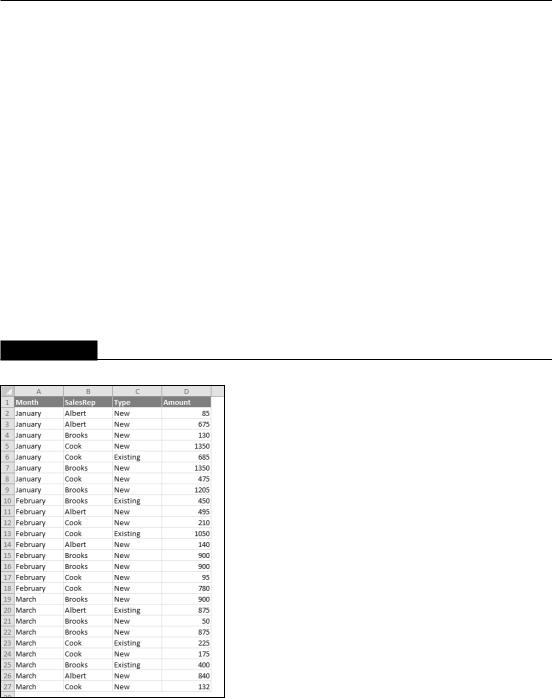
Figure 13.2 shows a simple worksheet that I use for the examples in this section. This sheet shows sales data categorized by Month, SalesRep, and Type. The worksheet contains named ranges that correspond to the labels in row 1.
On the CD
This workbook is available on the companion CD-ROM. The file is named multiple criteria counting
.xlsx.
Note
Several of the examples in this section use the COUNTIFS function, which was introduced in Excel 2007. I also present alternative versions of the formulas, which should be used if you plan to share your workbook with others who use an earlier version of Excel. n
FIGURE 13.2
This worksheet demonstrates various counting techniques that use multiple criteria.
288

Chapter 13: Creating Formulas That Count and Sum
Using And criteria
An And criterion counts cells if all specified conditions are met. A common example is a formula that counts the number of values that fall within a numerical range. For example, you may want to count cells that contain a value greater than 100 and less than or equal to 200. For this example, the COUNTIFS function will do the job:
=COUNTIFS(Amount,”>100”,Amount,”<=200”)
Note
If the data is contained in a table, you can use table referencing in your formulas. For example, if the table is named Table1, you can rewrite the preceding formula as:
=COUNTIFS(Table1[Amount],”>100”,Table1[Amount],”<=200”)
This method of writing formulas does not require named ranges. n
The COUNTIFS function accepts any number of paired arguments. The first member of the pair is the range to be counted (in this case, the range named Amount); the second member of the pair is the criterion. The preceding example contains two sets of paired arguments and returns the number of cells in which Amount is greater than 100 and less than or equal to 200.
Prior to Excel 2007, you would need to use a formula like this:
=COUNTIF(Amount,”>100”)-COUNTIF(Amount,”>200”)
The formula counts the number of values that are greater than 100 and then subtracts the number of values that are greater than or equal to 200. The result is the number of cells that contain a value greater than 100 and less than or equal to 200. This formula can be confusing because the formula refers to a condition “>200” even though the goal is to count values that are less than or equal to 200. Yet another alternate technique is to use an array formula, like the one that follows. You may find it easier to create this type of formula:
{=SUM((Amount>100)*(Amount<=200))}
Note
When you enter an array formula, remember to use Ctrl+Shift+Enter but don’t type the brackets. Excel includes the brackets for you. n
Sometimes, the counting criteria will be based on cells other than the cells being counted. You may, for example, want to count the number of sales that meet the following criteria:
•Month is January, and
•SalesRep is Brooks, and
•Amount is greater than 1000
289

Part II: Working with Formulas and Functions
The following formula (for Excel 2007 and Excel 2010) returns the number of items that meets all three criteria. Note that the COUNTIFS function uses three sets of pairs of arguments.
=COUNTIFS(Month,”January”,SalesRep,”Brooks”,Amount,”>1000”)
An alternative formula, which works with all versions of Excel, uses the SUMPRODUCT function. The following formula returns the same result as the previous formula.
=SUMPRODUCT((Month=”January”)*(SalesRep=”Brooks”)*(Amount>1000))
Yet another way to perform this count is to use an array formula:
{=SUM((Month=”January”)*(SalesRep=”Brooks”)*(Amount>1000))}
Using Or criteria
To count cells by using an Or criterion, you can sometimes use multiple COUNTIF functions. The following formula, for example, counts the number of sales made in January or February:
=COUNTIF(Month,”January”)+COUNTIF(Month,”February”)
You can also use the COUNTIF function in an array formula. The following array formula, for example, returns the same result as the previous formula:
{=SUM(COUNTIF(Month,{“January”,”February”}))}
But if you base your Or criteria on cells other than the cells being counted, the COUNTIF function won’t work. (Refer to Figure 13.2.) Suppose that you want to count the number of sales that meet the following criteria:
•Month is January, or
•SalesRep is Brooks, or
•Amount is greater than 1000
If you attempt to create a formula that uses COUNTIF, some double counting will occur. The solution is to use an array formula like this:
{=SUM(IF((Month=”January”)+(SalesRep=”Brooks”)+(Amount>1000),1))}
Combining And and Or criteria
In some cases, you may need to combine And and Or criteria when counting. For example, perhaps you want to count sales that meet the following criteria:
•Month is January, and
•SalesRep is Brooks, or SalesRep is Cook
290
Chapter 13: Creating Formulas That Count and Sum
This array formula returns the number of sales that meet the criteria:
{=SUM((Month=”January”)*IF((SalesRep=”Brooks”)+
(SalesRep=”Cook”),1))}
Counting the most frequently occurring entry
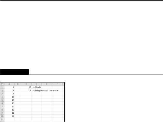
The MODE function returns the most frequently occurring value in a range. Figure 13.3 shows a worksheet with values in range A1:A10 (named Data). The formula that follows returns 10 because that value appears most frequently in the Data range:
=MODE(Data)
FIGURE 13.3
The MODE function returns the most frequently occurring value in a range.
To count the number of times the most frequently occurring value appears in the range (in other words, the frequency of the mode), use the following formula:
=COUNTIF(Data,MODE(Data))
This formula returns 5 because the modal value (10) appears five times in the Data range.
The MODE function works only for numeric values. It simply ignores cells that contain text. To find the most frequently occurring text entry in a range, you need to use an array formula.
To count the number of times the most frequently occurring item (text or values) appears in a range named Data, use the following array formula:
{=MAX(COUNTIF(Data,Data))}
This next array formula operates like the MODE function except that it works with both text and values:
{=INDEX(Data,MATCH(MAX(COUNTIF(Data,Data)),COUNTIF(Data,Data),0))}
291
Part II: Working with Formulas and Functions
Counting the occurrences of specific text
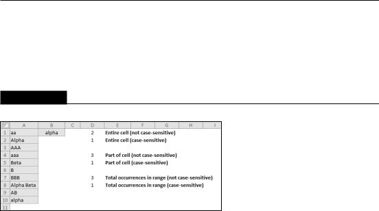
The examples in this section demonstrate various ways to count the occurrences of a character or text string in a range of cells. Figure 13.4 shows a worksheet used for these examples. Various text strings appear in the range A1:A10 (named Data); cell B1 is named Text.
FIGURE 13.4
This worksheet demonstrates various ways to count character strings in a range.
On the CD
The companion CD-ROM contains a workbook that demonstrates the formulas in this section. The file is named counting text in a range.xlsx.
Entire cell contents
To count the number of cells containing the contents of the Text cell (and nothing else), you can use the COUNTIF function as the following formula demonstrates.
=COUNTIF(Data,Text)
For example, if the Text cell contains the string Alpha, the formula returns 2 because two cells in the Data range contain this text. This formula is not case sensitive, so it counts both Alpha (cell A2) and alpha (cell A10). Note, however, that it does not count the cell that contains Alpha Beta (cell A8).
The following array formula is similar to the preceding formula, but this one is case sensitive:
{=SUM(IF(EXACT(Data,Text),1))}
Partial cell contents
To count the number of cells that contain a string that includes the contents of the Text cell, use this formula:
=COUNTIF(Data,”*”&Text&”*”)
292

Chapter 13: Creating Formulas That Count and Sum
For example, if the Text cell contains the text Alpha, the formula returns 3 because three cells in the Data range contain the text alpha (cells A2, A8, and A10). Note that the comparison is not case sensitive.
If you need a case-sensitive count, you can use the following array formula:
{=SUM(IF(LEN(Data)-LEN(SUBSTITUTE(Data,Text,””))>0,1))}
If the Text cells contain the text Alpha, the preceding formula returns 2 because the string appears in two cells (A2 and A8).
Total occurrences in a range
To count the total number of occurrences of a string within a range of cells, use the following array formula:
{=(SUM(LEN(Data))-SUM(LEN(SUBSTITUTE(Data,Text,””))))
/
LEN(Text)}
If the Text cell contains the character B, the formula returns 7 because the range contains seven instances of the string. This formula is case sensitive.
The following array formula is a modified version that is not case sensitive:
{=(SUM(LEN(Data))-SUM(LEN(SUBSTITUTE(UPPER(Data), UPPER(Text),””))))/LEN(Text)}
Counting the number of unique values
The following array formula returns the number of unique values in a range named Data:
{=SUM(1/COUNTIF(Data,Data))}
Note
The preceding formula is one of those “classic” Excel formulas that gets passed around the Internet. I don’t know who originated it. n
Useful as it is, this formula does have a serious limitation: If the range contains any blank cells, it returns an error. The following array formula solves this problem:
{=SUM(IF(COUNTIF(Data,Data)=0,””,1/COUNTIF(Data,Data)))}
Cross-Reference
To find out how to create an array formula that returns a list of unique items in a range, see Chapter 17. n
293

Part II: Working with Formulas and Functions
On the CD
The companion CD-ROM contains a workbook that demonstrates this technique. The file is named count unique.xlsx.
Creating a frequency distribution
A frequency distribution basically comprises a summary table that shows the frequency of each value in a range. For example, an instructor may create a frequency distribution of test scores. The table would show the count of A’s, B’s, C’s, and so on. Excel provides a number of ways to create frequency distributions. You can
•Use the FREQUENCY function.
•Create your own formulas.
•Use the Analysis ToolPak add-in.
•Use a pivot table.
On the CD
A workbook that demonstrates these four techniques appears on the companion CD-ROM. The file is named frequency distribution.xlsx.
The FREQUENCY function
Using the FREQUENCY function to create a frequency distribution can be a bit tricky. This function always returns an array, so you must use it in an array formula that’s entered into a multicell range.
Figure 13.5 shows some data in range A1:E25 (named Data). These values range from 1 to 500. The range G2:G11 contains the bins used for the frequency distribution. Each cell in this bin range contains the upper limit for the bin. In this case, the bins consist of <=50, 51–100, 101–150, and so on.
To create the frequency distribution, select a range of cells that corresponds to the number of cells in the bin range (in this example, select H2:H11 because the bins are in G2:G11). Then enter the following array formula into the selected range (press Ctrl+Shift+Enter it):
{=FREQUENCY(Data,G2:G11)}
The array formula returns the count of values in the Data range that fall into each bin. To create a frequency distribution that consists of percentages, use the following array formula:
{=FREQUENCY(Data,G2:G11)/COUNT(Data)}
Figure 13.6 shows two frequency distributions — one in terms of counts and one in terms of percentages. The figure also shows a chart (histogram) created from the frequency distribution.
294
Chapter 13: Creating Formulas That Count and Sum
FIGURE 13.5
Creating a frequency distribution for the data in A1:E25.
FIGURE 13.6
Frequency distributions created by using the FREQUENCY function.
295
Part II: Working with Formulas and Functions
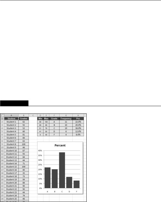
Using formulas to create a frequency distribution
Figure 13.7 shows a worksheet that contains test scores for 50 students in column B (the range is named Grades). Formulas in columns G and H calculate a frequency distribution for letter grades. The minimum and maximum values for each letter grade appear in columns D and E. For example, a test score between 80 and 89 (inclusive) earns a B. In addition, a chart displays the distribution of the test scores.
The formula in cell G2 that follows counts the number of scores that qualify for an A:
=COUNTIFS(Grades,”>=”&D2,Grades,”<=”&E2)
You may recognize this formula from a previous section in this chapter (see “Counting cells by using multiple criteria”). This formula was copied to the four cells below G2.
Note
The preceding formula uses the COUNTIFS function, which first appeared in Excel 2007. For compatibility with previous Excel versions, use this array formula:
{=SUM((Grades>=D2)*(Grades<=E2))}
FIGURE 13.7
Creating a frequency distribution of test scores.
296
Chapter 13: Creating Formulas That Count and Sum
The formulas in column H calculate the percentage of scores for each letter grade. The formula in H2, which was copied to the four cells below H2, is
=G2/SUM($G$2:$G$6)
Using the Analysis ToolPak to create a frequency distribution
The Analysis ToolPak add-in, distributed with Excel, provides another way to calculate a frequency distribution.
1.Enter your bin values in a range.
2.Choose Data Analysis Analysis to display the Data Analysis dialog box. If this command is not available, see the sidebar, “Is the Analysis ToolPak Installed?”.
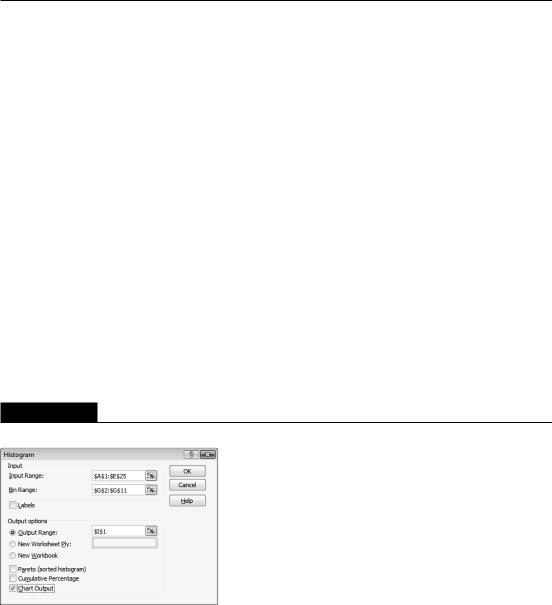
3.In the Data Analysis dialog box, select Histogram and then click OK. You should see the Histogram dialog box shown in Figure 13.8.
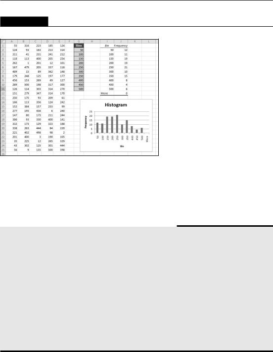
4.Specify the ranges for your data (Input Range), bins (Bin Range), and results (Output Range), and then select any options. Click OK. Figure 13.9 shows a frequency distribution (and chart) created with the Histogram option.
Caution
Note that the frequency distribution consists of values, not formulas. Therefore, if you make any changes to your input data, you need to rerun the Histogram procedure to update the results. n
FIGURE 13.8
The Analysis ToolPak’s Histogram dialog box.
297
Part II: Working with Formulas and Functions
FIGURE 13.9
A frequency distribution and chart generated by the Analysis ToolPak’s Histogram option.
Using a pivot table to create a frequency distribution
If your data is in the form of a table, you may prefer to use a pivot table to create a histogram. Figure 13.10 shows the student grade data summarized in a pivot table in columns D and E. The data bars were added using conditional formatting.
Is the Analysis ToolPak Installed?
To make sure that the Analysis ToolPak add-in is installed, click the Data tab. If the Ribbon displays the Data Analysis command in the Analysis group, you’re all set. If not, you’ll need to install the add-in:
1.Choose File Options to display the Excel Options dialog box.
2.Click the Add-ins tab on the left.
3.Select Excel Add-Ins from the Manage drop-down list.
4.Click Go to display the Add-Ins dialog box.
5.Place a check mark next to Analysis ToolPak.
6.Click OK.
If you’ve enabled the Developer tab, you can display the Add-Ins dialog box by choosing Developer Add-Ins Add-Ins.
Note: In the Add-Ins dialog box, you see an additional add-in, Analysis ToolPak - VBA. This add-in is for programmers, and you don’t need to install it.
298