

755
.pdf84 |
3G Evolution: HSPA and LTE for Mobile Broadband |
In case of base-station antennas in typical macro-cell environments (relatively large cells, relatively high base-station antenna positions, etc.), an antenna distance in the order of ten wavelengths is typically needed to ensure a low mutual fading correlation. At the same time, for a mobile terminal in the same kind of environment, an antenna distance in the order of only half a wavelength (0.5λ) is often sufficient to achieve relatively low mutual correlation [41]. The reason for the difference between the base station and the mobile terminal in this respect is that, in the macro-cell scenario, the multi-path reflections that cause the fading mainly occur in the near-zone around the mobile terminal. Thus, as seen from the mobile terminal, the different paths will typically arrive from a wide angle, implying a low fading correlation already with a relatively small antenna distance. At the same time, as seen from the (macro-cell) base station the different paths will typically arrive within a much smaller angle, implying the need for significantly larger antenna distance to achieve low fading correlation.1
On the other hand, in other deployment scenarios, such as micro-cell deployments with base-station antennas below roof-top level and indoor deployments, the environment as seen from the base station is more similar to the environment as seen from the mobile terminal. In such scenarios, a smaller base-station antenna distance is typically sufficient to ensure relatively low mutual correlation between the fading experienced by the different antennas.
The above discussion assumed antennas with the same polarization direction. Another means to achieve low mutual fading correlation is to apply different polarization directions for the different antennas [41]. The antennas can then be located relatively close to each other, implying a compact antenna arrangement, while still experiencing low mutual fading correlation.
6.2Benefits of multi-antenna techniques
The availability of multiple antennas at the transmitter and/or the receiver can be utilized in different ways to achieve different aims:
•Multiple antennas at the transmitter and/or the receiver can be used to provide additional diversity against fading on the radio channel. In this case, the channels experienced by the different antennas should have low mutual correlation, implying the need for a sufficiently large inter-antenna distance (spatial
1 Although the term ‘arrive’ is used above, the situation is exactly the same in case of multiple transmit antennas. Thus, in case of multiple base-station transmit antennas in a macro-cell scenario, the antenna distance typically needs to be a number of wavelengths to ensure low fading correlation while, in case of multiple transmit antennas at the mobile terminal, an antenna distance of a fraction of a wavelength is sufficient.

Multi-antenna techniques |
85 |
diversity), alternatively the use of different antenna polarization directions (polarization diversity).
•Multiple antennas at the transmitter and/or the receiver can be used to ‘shape’ the overall antenna beam (transmit beam and receive beam, respectively) in a certain way, for example, to maximize the overall antenna gain in the direction of the target receiver/transmitter or to suppress specific dominant interfering signals. Such beam-forming can be based either on high or low fading correlation between the antennas, as is further discussed in Section 6.4.2.
•The simultaneous availability of multiple antennas at the transmitter and the receiver can be used to create what can be seen as multiple parallel communication ‘channels’ over the radio interface. This provides the possibility for very high bandwidth utilization without a corresponding reduction in power efficiency or, in other words, the possibility for very high data rates within a limited bandwidth without an un-proportionally large degradation in terms of coverage. Herein we will refer to this as spatial multiplexing. It is often also referred to as MIMO (Multi-Input Multi-Output) antenna processing.
6.3Multiple receive antennas
Perhaps the most straightforward and historically the most commonly used multiantenna configuration is the use of multiple antennas at the receiver side. This is often referred to as receive diversity or RX diversity even if the aim of the multiple receive antennas is not always to achieve additional diversity against radio-channel fading.
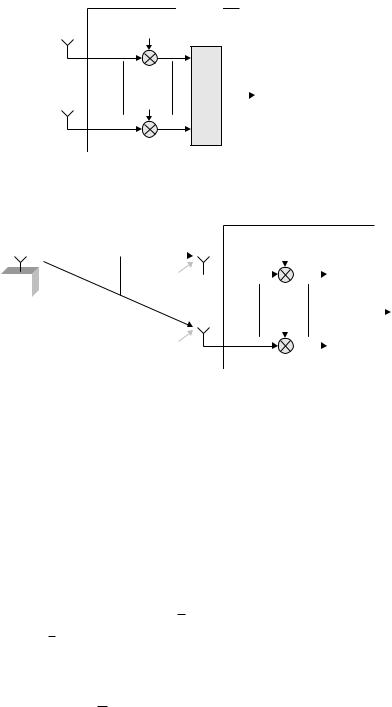
Figure 6.1 illustrates the basic principle of linear combining of signals r1, . . . , rNR received at NR different antennas, with the received signals being multiplied by complex weight factors w1, . . . , wNR before being added together. In vector notation this linear receive-antenna combining can be expressed as2
s w1 |
|
wNR |
|
.. |
|
|
wH r |
(6.1) |
|||
|
|
|
|
|
r1 |
|
|
|
|
|
|
|
· · · |
|
|
|
. |
|
|
|
|
|
|
ˆ = |
|
· |
|
|
= |
· |
|
|
|||
|
rNR |
|
|
||||||||
|
|
|
|
|
|
|
|
|
|
||
|
|
|
|
|
|
|
|
|
|
|
|
What is outlined in (6.1) and Figure 6.1 is linear receive-antenna combining in general. Different specific antenna-combining approaches then differ in the exact choice of the weight vector w.
2 Note that the weight factors are expressed as complex conjugates of w1, . . . , wNR .
86 |
3G Evolution: HSPA and LTE for Mobile Broadband |
Receiver
w1*
r1
wN* |
|
sˆ |
|
||
|
R |
|
rNR
Figure 6.1 Linear receive-antenna combining.
|
|
|
|
|
|
|
|
|
|
|
|
|
|
Receiver |
|
||
|
|
s |
|
h1 |
|
|
|
|
|
w1* |
|
|
|
|
|||
Base station or |
|
|
|
|
n1 |
|
|
r1 |
|
|
|
|
|
|
|||
|
|
|
|
|
|
|
|
|
|
|
|
||||||
|
|
|
|
|
|
|
|
|
|
|
|
|
|
|
|
||
TX |
|
|
|
|
|
|
|
|
|
|
|
|
|
|
|
||
mobile terminal |
|
|
|
|
|
|
|
|
|
|
|
|
|
|
|
|
|
|
|
|
hN |
|
|
|
|
|
|
|
|
|
|
|
|
ˆ |
|
Transmitter |
R |
|
|
|
|
|
|
|
|
|
|
|
|||||
|
|
|
|
|
|
wN* |
|
|
|
s |
|||||||
|
|
|
|
|
|
|
|
|
|
|
|
|
|
||||
|
|
|
|
|
|
|
|
|
|
|
|
R |
|
|
|
|
|
|
|
|
|
|
|
|
|
|
rN |
|
|
|
|
|
|
|
|
|
|
|
|
|
|
nN |
|
|
R |
|
|
|
|
||||
|
|
|
|
|
|
|
|
|
|
|
|
|
|||||
|
|
|
|
|
|
R |
|
|
|
|
|
|
|
|
|||
|
|
|
|
|
|
|
|
|
|
|
|
|
|
||||
|
|
|
|
|
|
|
|
|
|
|
|
|
|
|
|||
|
|
|
|
|
|
|
|
|
|
|
|
|
|
|
|
|
|
Figure 6.2 Linear receive-antenna combining.
Assuming that the transmitted signal is only subject to non-frequency-selective fading and (white) noise, i.e., there is no radio-channel time dispersion, the signals received at the different antennas in Figure 6.1 can be expressed as
r |
.. |
|
.. |
s |
.. |
|
h s n |
(6.2) |
||
|
r1 |
|
h1 |
|
n1 |
|
|
|
|
|
|
. |
|
. |
|
. |
|
|
|
|
|
|
= rNR |
|
= hNR |
· + nNR |
= · + |
|
||||
|
|
|
|
|
|
|
|
|
|
|
where s is the transmitted signal, the vector h consists of the NR complex channel gains, and the vector n consists of the noise impairing the signals received at the different antennas (see also Figure 6.2).
One can easily show that, to maximize the signal-to-noise ratio after linear combining, the weight vector w should be selected as [50]
|
MRC = |
h |
(6.3) |
w |

Multi-antenna techniques |
87 |
This is also known as Maximum-Ratio Combining (MRC). The MRC weights fulfill two purposes:
•Phase rotate the signals received at the different antennas to compensate for the corresponding channel phases and ensure that the signals are phase aligned when added together (coherent combining).
•Weight the signals in proportion to their corresponding channel gains, that is apply higher weights for stronger received signals.
In case of mutually uncorrelated antennas, that is sufficiently large antenna distances or different polarization directions, the channel gains h1, . . . , hNR are uncorrelated and the linear antenna combining provides diversity of order NR. In terms of receiver-side beam-forming, selecting the antenna weights according to (6.3) corresponds to a receiver beam with maximum gain NR in the direction of the target signal. Thus, the use of multiple receive antennas may increase the post-combiner signal-to-noise ratio in proportion to the number of receive antennas.
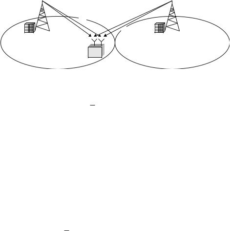
MRC is an appropriate antenna-combining strategy when the received signal is mainly impaired by noise. However, in many cases of mobile communication the received signal is mainly impaired by interference from other transmitters within the system, rather than by noise. In a situation with a relatively large number of interfering signals of approximately equal strength, maximum-ratio combining is typically still a good choice as, in this case, the overall interference will appear relatively ‘noise-like’ with no specific direction-of-arrival. However, in situations where there is a single dominating interferer (or, in the general case, a limited number of dominating interferers), as illustrated in Figure 6.3, improved performance can be achieved if, instead of selecting the antenna weights to maximize the received signal-to-noise ratio after antenna combining (MRC), the antenna weights are selected so that the interferer is suppressed. In terms of receiver-side beamforming this corresponds to a receiver beam with high attenuation in the direction of the interferer, rather than focusing the receiver beam in the direction of the target signal. Applying receive-antenna combining with a target to suppress specific interferers is often referred to as Interference Rejection Combining (IRC) [38].
In the case of a single dominating interferer as outlined in Figure 6.3, expression (6.2) can be extended according to
r |
.. |
|
.. |
s |
.. |
sI |
.. |
|
h s hI sI n (6.4) |
|||||
|
r1 |
|
h1 |
|
hI,1 |
|
n1 |
|
|
|
|
|
|
|
|
. |
|
. |
|
. |
|
. |
|
|
|
|
|
|
|
|
= rNR |
|
= hNR |
· + hI,NR |
· + nNR |
= · + · + |
||||||||
|
|
|
|
|
|
|
|
|
|
|
|
|
|
|
where sI is the transmitted interferer signal and the vector hI consists of the complex channel gains from the interferer to the NR receive antennas. By applying
88 |
3G Evolution: HSPA and LTE for Mobile Broadband |
s |
sI |
h1 |
hI,1 |
h2 |
hI,2 |
Target |
Interfering |
base station |
base station |
|
RX |
Figure 6.3 Downlink scenario with a single dominating interferer (special case of only two receive antennas).
expression (6.1) to (6.4) it is clear that the interfering signal will be completely suppressed if the weight vector w is selected to fulfill the expression
|
H · |
h |
I = 0 |
(6.5) |
w |
In the general case, (6.5) has NR − 1 non-trivial solutions, indicating flexibility in the weight-vector selection. This flexibility can be used to suppress additional dominating interferers. More specifically, in the general case of NR receive antennas there is a possibility to, at least in theory, completely suppress up to NR − 1 separate interferers. However, such a choice of antenna weights, providing complete suppression of a number of dominating interferers, may lead to a large, potentially very large, increase in the noise level after the antenna combining. This is similar to the potentially large increase in the noise level in case of a Zero-Forcing equalizer as discussed in Chapter 5.
Thus, similar to the case of linear equalization, a better approach is to select the antenna weight vector w to minimize the mean square error
ε = E{|ˆs − s|2} |
(6.6) |
also known as the Minimum Mean Square Error (MMSE) combining [41, 52].
Although Figure 6.3 illustrates a downlink scenario with a dominating interfering base station, IRC can also be applied to the uplink to suppress interference from specific mobile terminals. In this case, the interfering mobile terminal may either be in the same cell as the target mobile terminal (intra-cell-interference) or in a neighbor cell (inter-cell-interference) (see Figure 6.4a and b, respectively). Suppression of intra-cell interference is relevant in case of a non-orthogonal uplink, that is when multiple mobile terminals are transmitting simultaneously using the same time-frequency resource. Uplink intra-cell-interference suppression by means of IRC is sometimes also referred to as Spatial Division Multiple Access (SDMA) [68, 69].

Multi-antenna techniques |
89 |
|||||||
|
|
|
|
|
|
|
|
|
|
|
|
|
|
|
|
|
|
|
|
|
|
|
|
|
|
|
TX |
TX |
TX |
TX |
Interfering |
|
Interfering |
|
mobile terminal |
|
mobile terminal |
|
(a) |
|
(b) |
|
Figure 6.4 Receiver scenario with one strong interfering mobile terminal: (a) Intra-cell interference and (b) Inter-cell interference.
As discussed in Chapter 3, in practice a radio channel is always subject to at least some degree of time dispersion or, equivalently, frequency selectivity, causing corruption to a wide-band signal. As discussed in Chapter 5, one method to counteract such signal corruption is to apply linear equalization, either in the time or frequency domain.
It should be clear from the discussion above that linear receive-antenna combining has many similarities to linear equalization:
•Linear time-domain (frequency-domain) filtering/equalization as described in Chapter 5 implies that linear processing is applied to signals received at different time instances (different frequencies) with a target to maximize the postequalizer SNR (MRC-based equalization), alternatively to suppress signal corruption due to radio-channel frequency selectivity (zero-forcing equalization, MMSE equalization, etc.).
•Linear receive-antenna combining implies that linear processing is applied to signals received at different antennas, i.e. processing in the spatial domain, with a target to maximize the post-combiner SNR (MRC-based combining), alternatively to suppress specific interferers (IRC based on e.g. MMSE).
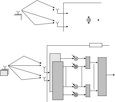
Thus, in the general case of frequency-selective channel and multiple receive antennas, two-dimensional time/space linear processing/filtering can be applied as illustrated in Figure 6.5 where the linear filtering can be seen as a generalization of the antenna weights of Figure 6.1. The filters should be jointly selected to minimize the overall impact of noise, interference and signal corruption due to radio-channel frequency selectivity.
Alternatively, especially in the case when cyclic-prefix insertion has been applied at the transmitter side, two-dimensional frequency/space linear processing can be applied as illustrated in Figure 6.6. The frequency-domain weights should then be jointly selected to minimize the overall impact of noise, interference, and signal corruption due to radio-channel frequency selectivity.
90 |
|
|
|
3G Evolution: HSPA and LTE for Mobile Broadband |
||||||||
|
|
|
|
|
|
|
|
|
|
|||
|
|
|
|
|
|
|
|
Receiver |
||||
|
|
|
|
|
Linear filtering |
|||||||
|
|
|
|
|
|
|
|
|
|
|
|
|
|
|
|
|
|
|
|
|
|
|
|
|
|
|
|
|
|
|
|
W1 |
|
|
|
sˆ |
|
|
|
|
|
|
|
|
|
|
|
||||
|
TX |
|
|
|
|
|
|
|
||||
|
|
|
|
|
|
|||||||
Base station or |
|
|
|
|
|
|
|
|
|
|||
mobile terminal |
|
|
W2 |
|
|
|
|
|
|
|||
|
|
|
|
|
|
|
|
|||||
|
|
|
|
|
|
|
|
|
|
|
|
|
Figure 6.5 Two-dimensional space/time linear processing (two receive antennas).
|
|
|
Receiver |
|
|
W*1,0 |
|
|
|
W*2,0 |
|
TX |
DFT |
|
sˆ |
Base station or |
|
W *1,N |
IDFT |
DFT |
|
||
mobile terminal |
1 |
||
|
|
C |
|
|
|
W *2,NC 1 |
|
Figure 6.6 Two-dimensional space/frequency linear processing (two receive antennas).
The frequency/space processing outlined in Figure 6.6, without the IDFT, is also applicable if receive diversity is to be applied to OFDM transmission. In the case of OFDM transmission, there is no signal corruption due to radio-channel frequency selectivity. Thus, the frequency-domain coefficients of Figure 6.6 can be selected taking into account only noise and interference. In principle, this means the antenna-combining schemes discussed above (MRC and IRC) are applied on a per-subcarrier basis.
Note that, although Figure 6.5 and Figure 6.6 assume two receive antennas, the corresponding receiver structures can straightforwardly be extended to more than two antennas.
6.4Multiple transmit antennas
As an alternative or complement to multiple receive antennas, diversity and beamforming can also be achieved by applying multiple antennas at the transmitter side. The use of multiple transmit antennas is primarily of interest for the downlink,
Multi-antenna techniques |
91 |
i.e. at the base station. In this case, the use of multiple transmit antennas provides an opportunity for diversity and beam-forming without the need for additional receive antennas and corresponding additional receiver chains at the mobile terminal. On the other hand, due to complexity reasons the use of multiple transmit antennas for the uplink, i.e. at the mobile terminal, is less attractive. In this case, it is typically preferred to apply additional receive antennas and corresponding receiver chains at the base station.
6.4.1 Transmit-antenna diversity
If no knowledge of the downlink channels of the different transmit antennas is available at the transmitter, multiple transmit antennas cannot provide beam-forming but only diversity. For this to be possible, there should be low mutual correlation between the channels of the different antennas. As discussed in Section 6.1, this can be achieved by means of sufficiently large distance between the antennas, alternatively by the use of different antenna polarization directions. Assuming such antenna configurations, different approaches can be taken to realize the diversity offered by the multiple transmit antennas.
6.4.1.1 Delay diversity
As discussed in Chapter 4, a radio channel subject to time dispersion, with the transmitted signal propagating to the receiver via multiple, independently fading paths with different delays, provides the possibility for multi-path diversity or, equivalently, frequency diversity. Thus multi-path propagation is actually beneficial in terms of radio-link performance, assuming that the amount of multi-path propagation is not too extensive and that the transmission scheme includes tools to counteract signal corruption due to the radio-channel frequency selectivity, for example, by means of OFDM transmission or the use of advanced receiver-side equalization.
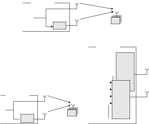
If the channel in itself is not time dispersive, the availability of multiple transmit antennas can be used to create artificial time dispersion or, equivalently, artificial frequency selectivity by transmitting identical signals with different relative delays from the different antennas. In this way, the antenna diversity, i.e. the fact that the fading experienced by the different antennas have low mutual correlation, can be transformed into frequency diversity. This kind of delay diversity is illustrated in Figure 6.7 for the special case of two transmit antennas. The relative delay T should be selected to ensure a suitable amount of frequency selectivity over the bandwidth of the signal to be transmitted. It should be noted that, although Figure 6.7 assumes two transmit antennas, delay diversity can straightforwardly be extended to more than two transmit antennas with different relative delays for each antenna.
Delay diversity is in essence invisible to the mobile terminal, which will simply see a single radio-channel subject to additional time dispersion. Delay diversity
92 |
3G Evolution: HSPA and LTE for Mobile Broadband |
BS transmitter
|
RX |
T |
Mobile terminal |
Figure 6.7 Two-antenna delay diversity.
BS transmitter
Cyclic
 shift
shift
(a)
BS transmitter a0  a1
a1  a2
a2  a3
a3 
|
|
a0 |
|
|
|
|
|
|
|
a1e j 2p f |
|
|
||
|
|
|||
a |
2 |
e j 2p f 2 |
|
OFDM |
|
||||
|
|
|
||
a3e j 2p f 3 |
|
modulation |
||
|
|
|||
RX
Mobile terminal
(b)
Figure 6.8 Two-antenna Cyclic-Delay Diversity (CDD).
can thus straightforwardly be introduced in an existing mobile-communication system without requiring any specific support in a corresponding radio-interface standard. Delay diversity is also applicable to basically any kind of transmission scheme that is designed to handle and benefit from frequency-selective fading, including, for example, WCDMA and CDMA2000.
6.4.1.2 Cyclic–delay diversity
Cyclic-Delay Diversity (CDD) [6] is similar to delay diversity with the main difference that cyclic delay diversity operates block-wise and applies cyclic shifts, rather than linear delays, to the different antennas (see Figure 6.8). Thus cyclicdelay diversity is applicable to block-based transmission schemes such as OFDM and DFTS-OFDM.
In case of OFDM transmission, a cyclic shift of the time-domain signal corresponds to a frequency-dependent phase shift before OFDM modulation, as illustrated in Figure 6.8b. Similar to delay diversity, this will create artificial frequency selectivity as seen by the receiver.

Multi-antenna techniques |
|
|
|
|
93 |
|||
|
BS transmitter |
|
|
|
|
h1 |
|
|
|
s0, s1, s2, s3, ... |
|
s0, s1, s2, s3, ... |
|
|
|||
|
STTD |
|
Mobile |
|||||
|
|
|
|
h2 |
|
|||
|
|
encoder |
|
|
|
RX |
||
|
|
s*, s*, s*, s*, ... |
terminal |
|||||
|
|
|
1 |
0 |
3 |
2 |
|
|
|
|
|
|
|
|
|
|
|
Sn, Sn 1  Sn* 1, Sn*
Figure 6.9 WCDMA Space–Time Transmit Diversity (STTD).
Also similar to delay diversity, CDD can straightforwardly be extended to more than two transmit antennas with different cyclic shifts for each antenna.
6.4.1.3 Diversity by means of space–time coding
Space-time coding is a general term used to indicate multi-antenna transmission schemes where modulation symbols are mapped in the time and spatial (transmit-antenna) domain to capture the diversity offered by the multiple transmit antennas. Two-antenna space–time block coding (STBC), more specifically a scheme referred to as Space–Time Transmit Diversity (STTD), has been part of the 3G WCDMA standard already from its first release [94].
As shown in Figure 6.9, STTD operates on pairs of modulation symbols. The modulation symbols are directly transmitted on the first antenna. However, on the second antenna the order of the modulation symbols within a pair is reversed. Furthermore, the modulation symbols are sign-reversed and complex-conjugated as illustrated in Figure 6.9.
In vector notation STTD transmission can be expressed as
|
|
= |
r2n+1 |
= |
h2 |
h1 |
· |
s2n+1 |
= |
|
· |
|
|
|
r |
|
r2n |
|
h1 |
−h2 |
|
s2n |
|
H |
|
s |
(6.7) |
where r2n and r2n+1 are the received symbols during the symbol intervals 2n and 2n + 1, respectively.3 It should be noted that this expression assumes that the channel coefficients h1 and h2 are constant over the time corresponding to two consecutive symbol intervals, an assumption that is typically valid. As the matrix H is a scaled unitary matrix, the sent symbols s2n and s2n+1 can be recovered from the received symbols r2n and r2n+1, without any interference between the symbols, by applying the matrix W = H−1 to the vector r.
3 Note that, for convenience, complex-conjugates have been applied for the second elements of r and s.