

755
.pdf64 |
3G Evolution: HSPA and LTE for Mobile Broadband |
Broadcast area
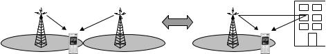
Figure 4.20 Broadcast scenario.
Broadcast |
Unicast |
(a) |
(b) |
Figure 4.21 Broadcast vs. Unicast transmission. (a) Broadcast and (b) Unicast.
information, or any other kind of information that, at a given time instant, may be of interest to a large number of people.
When the same information is to be provided to multiple mobile terminals within a cell it is often beneficial to provide this information as a single ‘broadcast’ radio transmission covering the entire cell and simultaneously being received by all relevant mobile terminals (Figure 4.21a), rather than providing the information by means of individual transmissions to each mobile terminal (unicast transmission, see Figure 4.21b).
As a broadcast transmission according to Figure 4.21a has to be dimensioned to reach also the worst-case mobile terminals, including mobile terminals at the cell border, it will be relative costly in terms of the recourses (base-station transmit power) needed to provide a certain broadcast-service data rate. Alternatively, taking into account the limited signal-to-noise ratio that can be achieved at, for example, the cell edge, the achievable broadcast data rates may be relatively limited, especially in case of large cells. One way to increase the broadcast data rates would then be to reduce the cell size, thereby increasing the cell-edge receive
OFDM transmission |
65 |
power. However, this will increase the number of cells to cover a certain area and is thus obviously negative from a cost-of-deployment point-of-view.
However, as discussed above, the provisioning of broadcast/multicast services in a mobile-communication network typically implies that identical information is to be provided over a large number of cells. In such a case, the resources (downlink transmit power) needed to provide a certain broadcast data rate can be considerably reduced if mobile terminals at the cell edge can utilize the received power from broadcast transmissions from multiple cells when detecting/decoding the broadcast data.
Especially large gains can be achieved if the mobile terminal can simultaneously receive and combine the broadcast transmissions from multiple cells before decoding. Such soft combining of broadcast/multicast transmissions from multiple cells has already been adopted for WCDMA Multimedia Broadcast/Multicast Service (MBMS) [102], as discussed in Chapter 11.
In case of WCDMA, each cell is transmitting on the downlink using different cell-specific scrambling codes (see Chapter 8). This is true also in case of MBMS. Thus the broadcast transmissions received from different cells are not identical but just provide the same broadcast/multicast information. As a consequence, the mobile terminal must still explicitly identify what cells to include in the soft combining. Furthermore, although the soft combining significantly increases the overall received power for mobile terminals at the cell border and thus significantly improve the overall broadcast efficiency, the broadcast transmissions from the different cells will still interfere with each other. This will limit the achievable broadcast-transmission signal-to-interference ratio and thus limit the achievable broadcast data rates.
One way to mitigate this and further improve the provisioning of broadcast/multicast services in a mobile-communication network is to ensure that the broadcast transmissions from different cells are truly identical and transmitted mutually time aligned. In this case, the transmissions received from multiple cells will, as seen from the mobile terminal, appear as a single transmission subject to severe multi-path propagation as illustrated in Figure 4.22. The transmission of identical time-aligned signals from multiple cells, especially in the case of provisioning of broadcast/multicast services, is sometimes referred to as Single-Frequency Network (SFN) operation [124].
In case of such identical time-aligned transmissions from multiple cells, the ‘intercell interference’ due to transmissions in neighboring cells will, from a terminal point of view, be replaced by signal corruption due to time dispersion. If the
66 |
3G Evolution: HSPA and LTE for Mobile Broadband |
Equivalence as seen from the mobile terminal
Figure 4.22 Equivalence between simulcast transmission and multi-path propagation.
broadcast transmission is based on OFDM with a cyclic prefix that covers the main part of this ‘time dispersion’, the achievable broadcast data rates are thus only limited by noise, implying that, especially in smaller cells, very high broadcast data rates can be achieved. Furthermore, in contrast to the explicit (in the receiver) multi-cell soft combining of WCDMA MBMS, the OFDM receiver does not need to explicitly identify the cells to be soft combined. Rather, all transmissions that fall within the cyclic prefix will ‘automatically’ be captured by the receiver.
5
Wider-band ‘single-carrier’ transmission
The previous chapters discussed multi-carrier transmission in general (Section 3.3.1) and OFDM transmission in particular (Chapter 4) as means to allow for very high overall transmission bandwidth while still being robust to signal corruption due to radio-channel frequency selectivity.
However, as discussed in the previous chapter, a drawback of OFDM modulation, as well as any kind of multi-carrier transmission, is the large variations in the instantaneous power of the transmitted signal. Such power variations imply a reduced power-amplifier efficiency and higher power-amplifier cost. This is especially critical for the uplink, due to the high importance of low mobile-terminal power consumption and cost.
As discussed in Chapter 4, several methods have been proposed on how to reduce the large power variations of an OFDM signal. However, most of these methods have limitations in terms of to what extent the power variations can be reduced. Furthermore, most of the methods also imply a significant computational complexity and/or a reduced link performance.
Thus, there is an interest to consider also wider-band single-carrier transmission as an alternative to multi-carrier transmission, especially for the uplink, i.e. for mobile-terminal transmission. It is then necessary to consider what can be done to handle the corruption to the signal waveform that will occur in most mobilecommunication environments due to radio-channel frequency selectivity.
5.1 Equalization against radio-channel frequency selectivity
Historically, the main method to handle signal corruption due to radio-channel frequency selectivity has been to apply different forms of equalization [50] at the receiver side. The aim of equalization is to, by different means, compensate for the channel frequency selectivity and thus, at least to some extent, restore the original signal shape.
67
68 |
3G Evolution: HSPA and LTE for Mobile Broadband |
5.1.1 Time-domain linear equalization
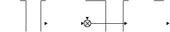
The most basic approach to equalization is the time-domain linear equalizer, consisting of a linear filter with an impulse response w(τ) applied to the received signal (see Figure 5.1).
By selecting different filter impulse responses, different receiver/equalizer strategies can be implemented. As an example, in DS-CDMA-based systems a so-called RAKE receiver structure has historically often been used. The RAKE receiver is simply the receiver structure of Figure 5.1 where the filter impulse response has been selected to provide channel-matched filtering
w(τ) = h (−τ), |
(5.1) |
that is the filter response has been selected as the complex conjugate of the timereversed channel impulse response. This is also often referred to as a MaximumRatio Combining (MRC) filter setting [50].
Selecting the receiver filter according to the MRC criterion, that is as a channelmatched filter, maximizes the post-filter signal-to-noise ratio (thus the term maximum-ratio combining). However, MRC-based filtering does not provide any compensation for any radio-channel frequency selectivity, that is no equalization. Thus, MRC-based receiver filtering is appropriate when the received signal is mainly impaired by noise or interference from other transmissions but not when a main part of the overall signal corruption is due to the radio-channel frequency selectivity.
Another alternative is to select the receiver filter to fully compensate for the radiochannel frequency selectivity. This can be achieved by selecting the receiver-filter impulse response to fulfill the relation
h(τ) w(τ) = 1 |
(5.2) |
where ‘ ’ denotes linear convolution. This selecting of the filter setting, also known as Zero-Forcing (ZF) equalization [50], provides full compensation for any radio-channel frequency selectivity (complete equalization) and thus full
Transmitter |
|
|
Channel model |
|
Receiver |
|||||
|
|
|
|
|
|
n(t ) |
|
|
|
|
|
|
s(t ) |
|
|
|
|
r(t) |
|
sˆ(t) |
|
|
|
|
|
|
|
|
||||
|
|
|
|
|
|
|||||
|
|
h(t) |
|
|
|
w(t) |
||||
|
|
|
|
|
|
|
|
|
||
|
|
|
|
|
|
|
|
|
||
|
|
|
|
|
|
|
|
|
|
|
Figure 5.1 General time-domain linear equalization.

Wider-band ‘single-carrier’ transmission |
69 |
suppression of any related signal corruption. However, zero-forcing equalization may lead to a large, potentially very large, increase in the noise level after equalization and thus to an overall degradation in the link performance. This will especially be the case when the channel has large variations in its frequency response.
A third and, in most cases, better alternative is to select a filter setting that provides a trade-off between signal corruption due to radio-channel frequency selectivity, and noise/interference. This can for example be done by selecting the filter to minimize the mean-square error between the equalizer output and the transmitted signal, i.e. to minimize
ε = E |
sˆ(t) − s(t) 2 |
(5.3) |
|
|
|
|
|
This is also referred to as a Minimum Mean-Square Error (MMSE) equalizer setting [50].
In practice, the linear equalizer has most often been implemented as a time-discrete FIR filter [52] with L filter taps applied to the sampled received signal, as illustrated in Figure 5.2. In general, the complexity of such a time-discrete equalizer grows relatively rapidly with the bandwidth of the signal to be equalized:
•A more wideband signal is subject to relatively more radio-channel frequency selectivity or, equivalently, relatively more time dispersion. This implies that the equalizer needs to have a larger span (larger length L, that is more filter taps) to be able to properly compensate for the channel frequency selectivity.
•A more wideband signal leads to a correspondingly higher sampling rate for the received signal. Thus also the receiver-filter processing needs to be carried out with a correspondingly higher rate.
Receiver nTs
r(t ) |
rn |
|
sˆn |
|
w |
||||
|
|
|
||
|
|
|
|
rn |
|
|
|
|
|
|
|
|
|
|
|
|
|||
D |
|
|
|
D |
|
D |
|
|
|
|
|||||
|
|
|
|
|
|
|
|
|
|
|
|
||||
|
|
|
|
|
|
|
|
|
|
|
|
|
|
||
|
|
|
|
|
|
|
|
|
|
|
|||||
|
w0 |
|
w1 |
|
|
wL 1 |
|
||||||||
|
|
|
|
|
|
|
|
|
|
|
|
|
|
|
sˆn |
|
|
|
|
|
|
|
|
|
|
|
|
|
|
|
|
|
|
|
|
|
|
|
|
|
|
|
|
||||
|
|
|
|
|
|
|
|
|
|
|
|||||
Figure 5.2 Linear equalization implemented as a time-discrete FIR filter.

70 |
|
|
3G Evolution: HSPA and LTE for Mobile Broadband |
||||
It can be |
shown [32] that the time-discrete |
MMSE equalizer setting |
|||||
|
= [w0, w1, . . . , wL−1]H is given by the expression |
|
|||||
w |
|
||||||
|
|
|
|
= R−1 |
|
|
(5.4) |
|
|
w |
p |
||||
In this expression, R is the channel-output auto-correlation matrix of size L × L, which depends on the channel impulse response as well as on the noise level, and p is the channel-output/channel-input cross-correlation vector of size L × 1 that depends on the channel impulse response.
Especially in case of a large equalizer span (large L), the time-domain MMSE equalizer may be of relatively high complexity:
•The equalization itself (the actual filtering) may be of relatively high complexity according to above.
•Calculation of the MMSE equalizer setting, especially the calculation of the inverse of the size L × L correlation matrix R, may be of relatively high
complexity.
5.1.2Frequency-domain equalization
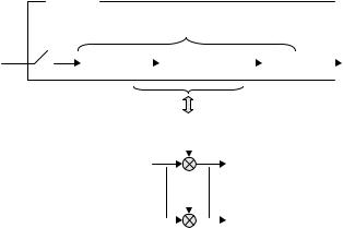
A possible way to reduce the complexity of linear equalization is to carry out the equalization in the frequency domain [24], as illustrated in Figure 5.3. In case of such frequency-domain linear equalization, the equalization is carried out blockwise with block size N. The sampled received signal is first transformed into the frequency domain by means of a size-N DFT. The equalization is then carried out as frequency-domain filtering, with the frequency-domain filter taps W0, . . . , WN−1, for example being the DFT of the corresponding time-domain filter taps w0, . . . , wL−1 of Figure 5.2. Finally, the equalized frequency-domain signal is transformed back to the time domain by means of a size-N inverse DFT. The block size-N should preferably be selected as N = 2n for some integer n to allow for computational-efficient radix-2 FFT/IFFT implementation of the DFT/IDFT processing.
For each processing block of size N, the frequency-domain equalization basically consists of:
•A size-N DFT/FFT.
•N complex multiplications (the frequency-domain filter).
•A size-N inverse DFT/FFT.
Especially in case of channels with extensive frequency selectivity, implying the need for a large span of a time-domain equalizer (large equalizer length L), equalization in the frequency domain according to Figure 5.3 can be of significantly less complexity, compared to time-domain equalization illustrated in Figure 5.2.
Wider-band ‘single-carrier’ transmission |
|
|
71 |
|||||||||||||
|
Receiver |
Block-wise processing |
|
|
|
|||||||||||
|
|
|
|
|
|
|||||||||||
|
|
|
(block-size N) |
|
|
|
|
|
||||||||
|
nTs |
Rk |
|
|
|
|
|
|
ˆ |
|
sˆn |
|||||
|
rn |
|
|
|
|
|
|
|
|
|||||||
r(t) |
DFT |
|
W |
|
|
Sk |
IDFT |
|||||||||
|
|
|
|
|
|
|
|
|
|
|
|
|||||
|
|
|
|
|
|
|
W0 |
|
|
|
|
|
|
|||
|
|
|
|
|
|
|
|
|
|
|
|
ˆ |
|
|
|
|
|
|
|
|
|
|
|
|
|
|
|
|
|
|
|
||
|
|
|
R0 |
|
|
|
||||||||||
|
|
|
S0 |
|
|
|
||||||||||
|
|
|
|
|
|
WN 1 |
|
|
|
|
|
|||||
|
|
|
|
|
|
|
|
|
|
|
|
ˆ |
|
|
|
|
|
|
|
|
|
|
|
|
|
|
|
|
|
|
|
||
|
|
|
RN 1 |
SN 1 |
|
|
|
|||||||||
Figure 5.3 Frequency-domain linear equalization.
However, there are two issues with frequency-domain equalization:
•The time-domain filtering of Figure 5.2 implements a time-discrete linear convolution. In contrast, frequency-domain filtering according to Figure 5.3 corresponds to circular convolution in the time domain. Assuming a time-
domain equalizer of length L, this implies that the first L − 1 samples at the output of the frequency-domain equalizer will not be identical to the corresponding output of the time-domain equalizer.
•The frequency-domain filter taps W0, . . . , WN−1 can be determined by first determining the pulse response of the corresponding time-domain filter and then transforming this filter into the frequency domain by means of a DFT. However, as mentioned above, determining e.g. the MMSE time-domain filter may be relative complex in case of a large equalizer length L.
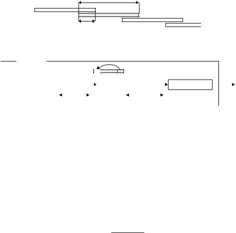
One way to address the first issue is to apply an overlap in the block-wise processing of the frequency-domain equalizer as outlined in Figure 5.4, where the overlap should be at least L − 1 samples. With such an overlap, the first L − 1 (‘incorrect’) samples at the output of the frequency-domain equalizer can be discarded as the corresponding samples are also (correctly) provided as the last part of the previously received/equalized block. The drawback with this kind of ‘overlap-and- discard’ processing is a computational overhead, that is somewhat higher receiver complexity.
An alternative approach that addresses both of the above issues is to apply cyclic-prefix insertion at the transmitter side (see Figure 5.5). Similar to OFDM, cyclic-prefix insertion in case of single-carrier transmission implies that a cyclic prefix of length NCP samples is inserted block-wise at the transmitter side. The
72 |
3G Evolution: HSPA and LTE for Mobile Broadband |
Processing block (N samples)
Overlap
( L 1 samples)
Figure 5.4 Overlap-and-discard processing.
Transmitter
Block-wise generation
Single-carrier |
|
|
|
|
|
CP |
|
|
|
|
|
|
|
|
x(t) |
|
|
|
|
|
|
|
|
|
|
|
|
D/A conversion |
|||
|
|
|
|
|
|
|
|
|
|
|
|
|
|||
signal generation |
|
|
|
|
|
insertion |
|
|
|
|
|
|
|
|
|
|
|
|
|
|
|
|
|
|
|
|
|
|
|
||
|
|
|
|
|
|
|
|
|
|||||||
|
|
N samples |
|
|
N NCP samples |
||||||||||
Figure 5.5 Cyclic-prefix insertion in case of single-carrier transmission.
transmitter-side block size should be the same as the block size N used for the receiver-side frequency-domain equalization.
With the introduction of a cyclic prefix, the channel will, from a receiver point of view, appear as a circular convolution over a receiver processing block of size N. Thus there is no need for any receiver overlap-and-discard processing. Furthermore, the frequency-domain filter taps can now be calculated directly from an estimate of the sampled channel frequency response without first determining the time-domain equalizer setting. As an example, in case of an MMSE equalizer the frequency-domain filter taps can be calculated according to
H
Wk = k (5.5)
|Hk|2 + N0
where N0 is the noise power and Hk is the sampled channel frequency response. For large equalizer lengths, this calculation is of much lower complexity compared to the time-domain calculation discussed in the previous section.
The drawback of cyclic-prefix insertion in case of single-carrier transmission is the same as for OFDM, that is it implies an overhead in terms of both power and bandwidth. One method to reduce the relative cyclic-prefix overhead is to increase the block size N of the frequency-domain equalizer. However, for the block-wise equalization to be accurate, the channel needs to be approximately constant over a time span corresponding to the size of the processing block. This constraint provides an upper limit on the block size N that depends on the rate of the channel variations. Note that this is similar to the constraint on the OFDM subcarrier spacing f = 1/Tu depending on the rate of the channel variations, as discussed in Chapter 4.

Wider-band ‘single-carrier’ transmission |
73 |
5.1.3 Other equalizer strategies
The previous sections discussed different approaches to linear equalization as a means to counter-act signal corruption of a wideband signal due to radio-channel frequency selectivity. However, there are also other approaches to equalization:
•Decision-Feedback Equalization (DFE) [50] implies that previously detected symbols are fed back and used to cancel the contribution of the corresponding transmitted symbols to the overall signal corruption. Such decision feedback is typically used in combination with time-domain linear filtering, where the linear filter transforms the channel response to a shape that is more suitable for the decision-feedback stage. Decision feedback can also very well be used in combination with frequency-domain linear equalization [24].
•Maximum-Likelihood (ML) detection, also known as Maximum Likelihood Sequence Estimation (MLSE), [25] is strictly speaking not an equalization scheme but rather a receiver approach where the impact of radio-channel time dispersion is explicitly taken into account in the receiver-side detection process. Fundamentally, an ML detector uses the entire received signal to decide on the most likely transmitted sequence, taking into account the impact of the time dis-
persion on the received signal. To implement maximum-likelihood detection the Viterbi algorithm [26] is often used.1 However, although maximum-likelihood
detection based on the Viterbi algorithm has been extensively used for 2G mobile communication such as GSM, it is foreseen to be too complex to be applied for the 3G evolution due to the much wider transmission bandwidth leading to both much more extensive channel frequency selectivity and much higher sampling rates.
5.2Uplink FDMA with flexible bandwidth assignment
In practice, there are obviously often multiple mobile terminals within a cell and thus multiple mobile terminals that should share the overall uplink radio resource within the cell by means of the uplink intra-cell multiple-access scheme.
In case of mobile communication based on WCDMA and cdma2000, uplink transmissions within a cell are mutually non-orthogonal and the base-station receiver relies on the processing gain due to channel coding and additional direct-sequence spreading to suppress the intra-cell interference. Although non-orthogonal multiple access can, fundamentally, provide higher capacity compared to orthogonal multiple access, in practice the possibility for mutually orthogonal uplink transmissions within a cell is often beneficial from a system-performance point-of-view.
1 Thus the term ‘Viterbi equalizer’ is sometimes used for the ML detector.