

3G Evolution. HSPA and LTE for Mobile Broadband
.pdfHigh data rates in mobile communication |
43 |
Power density (dBm /30 kHz)
30.0 |
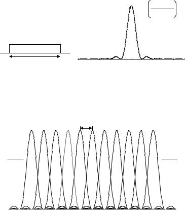
3.84 MHz |
20.0
10.0
0.0
10.0
20.0
30.0
40.0 


 2.5 2.0 1.5 1.0 0.5 0.0 0.5 1.0 1.5 2.0 2.5
Frequency (MHz)
|
|
|
|
|
|
1 |
|
|
f f1 |
||
p(f ) |
1 |
|
p( f f1) |
f1 f f2 |
|||||||
|
2 |
1 cos |
|
|
fcr a |
|
|||||
|
|
|
|
|
|
0 |
|
|
f f2 |
||
f |
f |
cr |
(1 a) |
f f |
cr |
(1 a) |
|
||||
1 |
|
|
|
2 |
2 |
|
2 |
|
|
||
BW 2 f2 fcr (1 a) 4.7 MHz
Figure 3.6 Theoretical WCDMA spectrum. Raised-cosine shape with roll-off α = 0.22.
inter-subcarrier interference. It should be noted though that a smaller subcarrier spacing can be used with only limited inter-subcarrier interference.
A second drawback of multi-carrier transmission is that, similar to the use of higher-order modulation, the parallel transmission of multiple carriers will lead to larger variations in the instantaneous transmit power. Thus, similar to the use of higher-order modulation, multi-carrier transmission will have a negative impact on the transmitter power-amplifier efficiency, implying increased transmitter power consumption and increased power-amplifier cost. Alternatively, the average transmit power must be reduced, implying a reduced range for a given data rate. For this reason, similar to the use of higher-order modulation, multi-carrier transmission is more suitable for the downlink (base-station transmission), compared to the uplink (mobile-terminal transmission), due to the higher importance of high power-amplifier efficiency at the mobile terminal.
The main advantage with the kind of multi-carrier extension outlined in Figure 3.5 is that it provides a very smooth evolution, in terms of both radio equipment and spectrum, of an already existing radio-access technology to wider transmission bandwidth and a corresponding possibility for higher data rates, especially for the downlink. In essence this kind of multi-carrier evolution to wider bandwidth can be designed so that, for legacy terminals not capable of multi-carrier reception, each downlink ‘subcarrier’ will appear as an original, more narrowband carrier, while, for a multi-carrier-capable terminal, the network can make use of the full multi-carrier bandwidth to provide higher data rates.
The next chapter will discuss, in more detail, a different approach to multi-carrier transmission, based on so-called OFDM technique.
4
OFDM transmission
In this chapter, a more detailed overview of OFDM or Orthogonal Frequency Division Multiplexing will be given. OFDM has been adopted as the downlink transmission scheme for the 3GPP Long-Term Evolution (LTE) and is also used for several other radio technologies, e.g. WiMAX [116] and the DVB broadcast technologies [17].
4.1 Basic principles of OFDM
Transmission by means of OFDM can be seen as a kind of multi-carrier transmission. The basic characteristics of OFDM transmission, which distinguish it from a straightforward multi-carrier extension of a more narrowband transmission scheme as outlined in Figure 3.5 in the previous chapter, are:
•The use of a relatively large number of narrowband subcarriers. In contrast, a straightforward multi-carrier extension as outlined in Figure 3.5 would typically consist of only a few subcarriers, each with a relatively wide bandwidth. As an example, a WCDMA multi-carrier evolution to a 20 MHz overall transmission bandwidth could consist of four (sub)carriers, each with a bandwidth in the order of 5 MHz. In comparison, OFDM transmission may imply that several hundred subcarriers are transmitted over the same radio link to the same receiver.
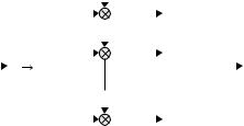
•Simple rectangular pulse shaping as illustrated in Figure 4.1a. This corresponds to a sinc-square-shaped per-subcarrier spectrum, as illustrated in Figure 4.1b.
•Tight frequency-domain packing of the subcarriers with a subcarrier spacing f = 1/Tu, where Tu is the per-subcarrier modulation-symbol time (see Figure 4.2). The subcarrier spacing is thus equal to the per-subcarrier modulation rate 1/Tu.
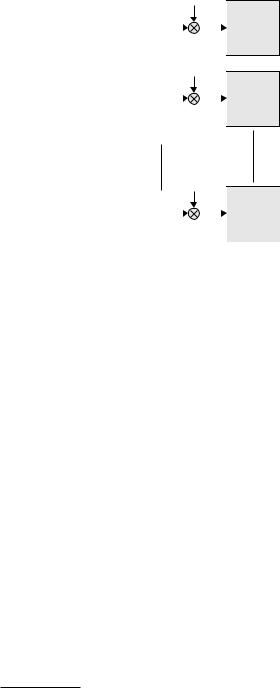
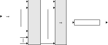
An illustrative description of a basic OFDM modulator is provided in Figure 4.3. It consists of a bank of Nc complex modulators, where each modulator corresponds to one OFDM subcarrier.
45
46 |
3G Evolution: HSPA and LTE for Mobile Broadband |
|
|
|
2 |
|
|
sin(pf/ f ) |
|
Subcarrier |
(pf/ f ) |
|
spectrum |
|
Pulse shape |
|
|
Tu 1/ f |
4 f 3 f 2 f f 0 |
f 2 f 3 f 4 f |
Time domain |
Frequency domain |
|
(a) |
(b) |
|
Figure 4.1 Per-subcarrier pulse shape and spectrum for basic OFDM transmission.
f 1/Tu
Figure 4.2 OFDM subcarrier spacing.
In complex baseband notation, a basic OFDM signal x(t) during the time interval mTu ≤ t < (m + 1)Tu can thus be expressed as
|
Nc−1 |
Nc−1 |
(m) |
|
j2πk ft |
|
|
|
|
|
|
||
x(t) = |
xk(t) = |
k=0 |
ak |
e |
|
(4.1) |
|
k=0 |
|
|
|
|
where xk(t) is the kth modulated subcarrier with frequency fk = k · f and ak(m) is the, in general complex, modulation symbol applied to the kth subcarrier during the mth OFDM symbol interval, i.e. during the time interval mTu ≤ t < (m + 1)Tu. OFDM transmission is thus block based, implying that, during each OFDM symbol interval, Nc modulation symbols are transmitted in parallel. The modulation symbols can be from any modulation alphabet, such as QPSK, 16QAM, or 64QAM.
OFDM transmission |
|
|
|
|
|
|
|
|
|
|
|
47 |
||||||
|
|
|
|
|
|
|
a0m |
e j2pf0t |
|
|
|
|
|
|
||||
|
|
|
|
|
|
|
|
|
|
|
x0(t) |
|
|
|
||||
|
|
|
|
|
|
|
|
|
|
|
|
|
|
|||||
|
|
|
|
|
|
|
|
|
|
|
|
|
|
|
|
|
|
|
|
|
|
|
|
|
|
am |
e j2pf1t |
|
|
|
|
|
|
||||
|
m |
m |
m |
|
|
|
|
|
|
x |
|
(t) |
|
|
|
|||
|
|
|
|
|
|
|
|
|
|
|
||||||||
|
|
|
1 |
|
1 |
|
|
|
|
|
||||||||
|
a0 |
, a1 |
, ..., aNc 1 |
S |
P |
|
|
|
|
|
|
|
|
|
|
x(t) |
||
|
aNm |
1 e |
j2pfN 1t |
|
|
|
||||||||||||
|
|
|
|
|
|
|
|
|
|
|||||||||
|
|
|
|
|
|
|
|
|
|
|
|
|
||||||
|
|
|
|
|
|
|
|
|
|
c xN |
1(t) |
|
|
|
||||
|
|
|
|
|
|
|
|
|
|
|
|
|
||||||
|
|
|
|
|
|
|
c |
|
|
|
|
c |
|
|
|
|
|
|
|
|
|
|
|
|
|
|
|
|
|
|
|
|
|
|
|
|
|
fk k f
Figure valid for time interval mTu t (m 1)Tu
Figure 4.3 OFDM modulation.
The number of OFDM subcarriers can range from less than one hundred to several thousand, with the subcarrier spacing ranging from several hundred kHz down to a few kHz. What subcarrier spacing to use depends on what types of environments the system is to operate in, including such aspects as the maximum expected radiochannel frequency selectivity (maximum expected time dispersion) and the maximum expected rate of channel variations (maximum expected Doppler spread). Once the subcarrier spacing has been selected, the number of subcarriers can be decided based on the assumed overall transmission bandwidth, taking into account acceptable out-of-band emission, etc. The selection of OFDM subcarrier spacing and number of subcarriers is discussed in somewhat more detail in Section 4.8.
As an example, for 3GPP LTE the basic subcarrier spacing equals 15 kHz. On the other hand, the number of subcarriers depends on the transmission bandwidth, with in the order of 600 subcarriers in case of operation in a 10 MHz spectrum allocation and correspondingly fewer/more subcarriers in case of smaller/larger overall transmission bandwidths.
The term Orthogonal Frequency Division Multiplex is due to the fact that two modulated OFDM subcarriers xk1 (t) and xk2 (t) are mutually orthogonal over the time interval mTu ≤ t < (m + 1)Tu, i.e.
(m+1)Tu |
(m+1)Tu |
x |
k1 |
(t)x (t) dt |
= |
a |
k1 |
a e j2πk1 fte−j2πk2 ft dt |
= |
0 for k |
1 = |
k |
2 |
mTu |
k2 |
mTu |
k2 |
|
|
||||||
|
|
|
|
|
|
|
|
|
|
(4.2) Thus basic OFDM transmission can be seen as the modulation of a set of orthogonal functions ϕk(t), where
ϕk(t) |
= |
|
e j2πk ft |
0 ≤ t < Tu |
(4.3) |
|
0 |
otherwise |
|
48 |
|
|
|
3G Evolution: HSPA and LTE for Mobile Broadband |
|
number) |
|
ak(m) |
|
|
Nc 1 |
|
||
|
|
|
|
|
|
(subcarrier |
Nc 2 |
|
|
|
|
|
|
|
Frequency |
k |
|
|
|
|
|
|
|
|
1 |
|
|
|
|
0 |
|
|
|
|
|
m 2 m 1 m |
m 1 m 2 |
||
Time (OFDM symbol number)
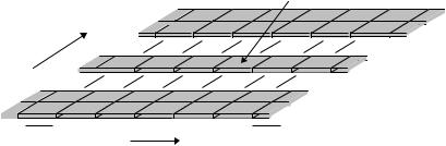
Figure 4.4 OFDM time–frequency grid.
The ‘physical resource’ in case of OFDM transmission is often illustrated as a time–frequency grid according to Figure 4.4 where each ‘column’ corresponds to one OFDM symbol and each ‘row’ corresponds to one OFDM subcarrier.
4.2OFDM demodulation
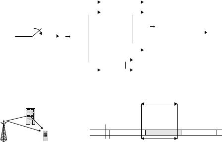
Figure 4.5 illustrates the basic principle of OFDM demodulation consisting of a bank of correlators, one for each subcarrier. Taking into account the orthogonality between subcarriers according to (4.2), it is clear that, in the ideal case, two OFDM subcarriers do not cause any interference to each other after demodulation. Note that this is the case despite the fact that the spectrum of neighbor subcarriers clearly overlap, as can be seen from Figure 4.2. Thus the avoidance of interference between OFDM subcarriers is not simply due to a subcarrier spectrum separation, which is, for example, the case for the kind of straightforward multi-carrier extension outlined in Figure 3.5 in the previous chapter. Rather, the subcarrier orthogonality is due to the specific frequency-domain structure of each subcarrier in combination with the specific choice of a subcarrier spacing f equal to the per-subcarrier symbol rate 1/Tu. However, this also implies that, in contrast to the kind of multi-carrier transmission outlined in Section 3.3.1 of the previous chapter, any corruption of the frequency-domain structure of the OFDM subcarriers, e.g. due to a frequencyselective radio channel, may lead to a loss of inter-subcarrier orthogonality and thus to interference between subcarriers. To handle this and to make an OFDM signal truly robust to radio-channel frequency selectivity, cyclic-prefix insertion is typically used, as will be further discussed in Section 4.4.
4.3OFDM implementation using IFFT/FFT processing
Although a bank of modulators/correlators according to Figures 4.3 and 4.5 can be used to illustrate the basic principles of OFDM modulation and demodulation, respectively, these are not the most appropriate modulator/demodulator structures
OFDM transmission |
49 |
|
e j2pf0t |
|
(m 1)Tu |
|||
|
|
|||||
|
|
|
|
|
|
... |
|
|
|
|
|||
|
|
|
|
|
|
mTu |
|
e j2pf1t |
|
(m 1)Tu |
|||
|
|
|||||
|
|
|
|
|
|
|
r(t) |
|
|
|
|
|
... |
|
|
|
||||
|
|
|
|
|
mTu |
|
|
|
|
|
|
|
|
|
e j2pfNc 1t |
|
(m 1)Tu |
||
|
|||||
|
|
||||
|
|
|
|
|
|
|
|
|
|
|
... |
|
|
|
|
||
|
fk k f |
|
mTu |
||
Figure 4.5 Basic principle of OFDM demodulation.
 aˆ0(m)
 aˆ1(m)

 aˆ(Nmc) 1
for actual implementation. Actually, due to its specific structure and the selection of a subcarrier spacing f equal to the per-subcarrier symbol rate 1/Tu, OFDM allows for low-complexity implementation by means of computationally efficient
Fast Fourier Transform (FFT) processing.
To confirm this, consider a time-discrete (sampled) OFDM signal where it is assumed that the sampling rate fs is a multiple of the subcarrier spacing f , i.e. fs = 1/Ts = N · f . The parameter N should be chosen so that the sampling theorem [50] is sufficiently fulfilled.1 As Nc · f can be seen as the nominal bandwidth of the OFDM signal, this implies that N should exceed Nc with a sufficient margin.
With these assumptions, the time-discrete OFDM signal can be expressed as2
|
|
|
|
|
Nc−1 |
e j2πk fnTs |
|
Nc−1 |
|
e j2πkn/N |
|
N−1 |
e j2πkn/N |
|
|
|
|
|
|
|
|
|
|
|
|
|
|||
x |
n = |
x(nT |
) |
= |
a |
= |
a |
= |
a |
(4.4) |
||||
|
s |
|
k |
|
k=0 |
k |
|
k |
|
|
||||
where |
|
|
|
k=0 |
|
|
|
|
|
k=0 |
|
|
||
|
|
|
|
ak = |
0k |
Nc≤ |
|
k < N |
|
|
|
(4.5) |
||
|
|
|
|
|
|
|
|
|
|
|||||
|
|
|
|
|
|
|
a |
0 |
k < Nc |
|
|
|
|
|
≤
1 An OFDM signal defined according to (4.1) in theory has an infinite bandwidth and thus the sampling theorem can never be fulfilled completely.
2 From now on the index m on the modulation symbols, indicating the OFDM-symbol number, will be ignored unless especially needed.
50 |
|
|
|
|
|
|
|
|
3G Evolution: HSPA and LTE for Mobile Broadband |
|||||||||
|
|
|
|
|
|
a0 |
|
x0 |
|
|
|
|
|
|
|
|||
|
|
|
|
|
|
|
|
|
|
|
|
|
|
|
|
|
||
|
|
|
|
|
|
a1 |
x1 |
|
|
|
|
|
|
|||||
|
a0, a1, ..., aN |
1 |
|
|
|
|
|
|
|
|
|
|
|
|
|
|
|
|
|
|
|
|
|
|
|
|
|
|
|
|
|
|
|
|
|
||
|
c |
|
|
S |
P |
|
|
|
|
|
|
|
|
|
|
|
|
|
|
|
|
|
|
|
|
Size-N |
|
|
|
|
|
|
|
x(t) |
|||
|
|
|
|
|
|
|
|
|
|
|
|
|
|
|
|
|||
|
|
|
|
|
|
|
|
|
|
|
|
|
|
|
D/A conversion |
|||
|
|
|
|
|
|
|
|
|
IDFT |
|
|
P S |
|
|
|
|
|
|
|
|
|
|
|
|
|
|
|
|
|
|
|
||||||
|
|
|
|
|
|
aN |
1 |
|
(IFFT) |
|
|
|
|
|
|
|
|
|
|
|
|
|
|
|
|
|
|
|
|
|
|
|
|
|
|
||
|
|
|
|
|
|
c |
|
|
|
|
|
|
|
|
|
|
|
|
|
|
|
|
|
|
|
|
|
|
|
|
|
|
|
|
|
|
|
0
xN 1
0
Figure 4.6 OFDM modulation by means of IFFT processing.
Thus, the sequence xn, i.e. the sampled OFDM signal, is the size-N Inverse Discrete Fourier Transform (IDFT) of the block of modulation symbols a0, a1, . . . , aNc − 1 extended with zeros to length N. OFDM modulation can thus be implemented by means of IDFT processing followed by digital-to-analog conversion, as illustrated in Figure 4.6. Especially, by selecting the IDFT size N equal to 2m for some integer m, the OFDM modulation can be implemented by means of implementationefficient radix-2 Inverse Fast Fourier Transform (IFFT) processing. It should be noted that the ratio N/Nc, which could be seen as the over-sampling of the timediscrete OFDM signal, could very well be, and typically is, a non-integer number. As an example and as already mentioned, for 3GPP LTE the number of subcarriers Nc is approximately 600 in case of a 10 MHz spectrum allocation. The IFFT size can then, for example, be selected as N = 1024. This corresponds to a sampling rate fs = N · f = 15.36 MHz, where f = 15 kHz is the LTE subcarrier spacing.
It is important to understand that IDFT/IFFT-based implementation of an OFDM modulator, and even more so the exact IDFT/IFFT size, are just transmitterimplementation choices and not something that would be mandated by any radio-access specification. As an example, nothing forbids the implementation of an OFDM modulator as a set of parallel modulators as illustrated in Figure 4.3. Also nothing prevents the use of a larger IFFT size, e.g. a size-2048 IFFT size, even in case of a smaller number of OFDM subcarriers.
Similar to OFDM modulation, efficient FFT processing can be used for OFDM demodulation, replacing the bank of Nc parallel demodulators of Figure 4.5 with sampling with some sampling rate fs = 1/Ts, followed by a size-N DFT/FFT, as illustrated in Figure 4.7.
OFDM transmission |
|
|
|
|
|
|
|
|
|
|
|
|
|
|
51 |
|
|
|
|
|
r0 |
|
aˆ0 |
|
|
|
|
|
|
|
|||
|
|
|
|
|
|
|
|
|
|
|
|
|
|
|
|
|
|
|
|
|
r1 |
|
aˆ1 |
|
|
|
|
|
|
|
|||
nTs |
|
|
|
|
|
|
|
|
|
P S |
aˆ |
0 |
, aˆ |
1 |
, ..., aˆ |
|
|
|
|
|
|
|
|
|
|
||||||||
r(t) |
rn |
|
|
|
Size-N |
|
|
|
|
|
Nc 1 |
|||||
|
|
|
|
|
|
|
|
|
|
|
|
|
||||
|
|
|
S P |
|
|
DFT |
|
|
|
|
|
|
|
|
|
|
|
|
|
|
|
|
|
|
|
|
|
|
|
|
|
||
|
|
|
|
|
|
(FFT) |
aˆNc 1 |
|
|
|
|
|
|
|
||
|
|
|
|
|
|
|
|
|
|
|
|
|
|
|||
|
|
|
|
rN 1 |
|
|
|
|
|
|
|
|
|
|
|
|
|
|
|
|
|
|
Unused |
|
|
|
|
|
|
||||
|
|
|
|
|
|
|
|
|
|
|
|
|||||
|
|
|
|
|
|
|
|
|
|
|
|
|
|
|
|
|
Figure 4.7 OFDM demodulation by means of FFT processing.
Tu
t |
Direct path |
|
(m 1) |
(m) |
(m 1) |
|
|
ak |
ak |
ak |
|
|
|
|
|
|
Reflected path t
Integration interval for demodulation of direct path
Figure 4.8 Time dispersion and corresponding received-signal timing.
4.4 Cyclic-prefix insertion
As described in Section 4.2, an uncorrupted OFDM signal can be demodulated without any interference between subcarriers. One way to understand this subcarrier orthogonality is to recognize that a modulated subcarrier xk(t) in (4.1) consists of an integer number of periods of complex exponentials during the demodulator integration interval Tu = 1/f .
However, in case of a time-dispersive channel the orthogonality between the subcarriers will, at least partly, be lost. The reason for this loss of subcarrier orthogonality in case of a time-dispersive channel is that, in this case, the demodulator correlation interval for one path will overlap with the symbol boundary of a different path, as illustrated in Figure 4.8. Thus, the integration interval will not necessarily correspond to an integer number of periods of complex exponentials of that path as the modulation symbols ak may differ between consecutive symbol intervals. As a consequence, in case of a time-dispersive channel there will not only be inter-symbol interference within a subcarrier but also interference between subcarriers.
Another way to explain the interference between subcarriers in case of a timedispersive channel is to have in mind that time dispersion on the radio channel
52 |
|
|
|
|
|
|
|
|
|
|
|
|
|
3G Evolution: HSPA and LTE for Mobile Broadband |
|||||||||||||||||||
|
|
|
|
|
|
|
|
|
|
|
|
|
|
|
Copy and insert |
|
|
|
|
|
|
|
|
||||||||||
|
|
|
|
a0 |
|
|
|
|
|
|
|
|
|
|
|
|
|
|
|
|
|
|
|
|
|
|
|
|
|
|
|
|
|
|
|
|
|
|
|
|
|
|
|
|
|
|
|
|
|
|
|
|
|
|
|
|
|
|
|
|
|
|
|
|
|
|
|
|
|
|
|
|
|
|
|
|
|
|
|
|
|
|
|
|
|
|
|
|
|
|
|
|
|
|
|
|
|
|
|
|
|
|
|
|
|
|
|
OFDM |
|
|
|
|
|
|
|
|
|
|
|
|
|
|
|
|
|
|
|
|
|
|
|
|
|
|
|
|
|
|
|
|
|
|
|
|
|
|
|
|
|
|
|
|
|
|
|
|
|
|
|
|
|
|
|
|
|
|
|
||
|
|
|
|
|
|
|
|
|
|
|
|
|
|
|
|
|
|
|
|
|
|
|
|
|
|
|
|
||||||
|
|
|
|
|
|
|
|
|
|
CP |
|
|
|
|
|
|
|
|
|
|
|
|
|||||||||||
|
|
|
|
|
|
|
mod. |
|
|
|
|
|
|
|
|
|
|
|
|
|
|
|
|
|
|
|
|
|
|
|
|||
|
|
|
|
|
|
|
|
|
|
|
|
|
|
|
|
|
insertion |
|
|
|
|
|
|
|
|
|
|
|
|
||||
|
|
aNc 1 |
|
|
(IFFT ) |
|
|
|
|
|
|
|
|
|
|
|
|
|
|
|
|
|
|
|
|
|
|
||||||
|
|
|
|
|
|
|
|
|
|
|
|
|
|
|
|
|
|
|
|
|
|
|
|
|
|
||||||||
|
|
|
|
Tu |
|
|
|
|
|
|
|
|
|
|
|
Tu Tcp |
|||||||||||||||||
|
|
|
|
|
|
|
|
|
|
|
|
|
|
||||||||||||||||||||
|
|
|
|
|
|
|
|
(N samples) |
|
|
|
|
|
|
|
|
(N NCP samples) |
||||||||||||||||
|
|
|
|
t |
|
|
Direct path |
|
|
|
|
|
|
|
|
|
|
|
TCP |
|
Tu |
||||||||||||
|
|
|
|
|
|
|
|
|
|
|
|
|
|
|
|
|
|
||||||||||||||||
|
|
|
|
|
|
|
|
|
|
|
|
|
|
|
|
|
|
|
|
|
|
|
|
|
|
|
|
|
|
||||
|
|
|
|
|
|
|
|
|
|
|
|
|
|
|
|
|
|
|
|
|
|
|
|
|
|
|
|
|
|
||||
|
|
|
|
|
|
|
|
|
|
|
|
|
|
|
|
|
|
|
|
|
|
|
|
|
|
|
|
|
|
||||
|
|
|
|
|
|
|
|
|
|
|
|
|
|
|
|
|
|
|
|
|
|
|
|
|
|
|
|
|
|
||||
|
|
|
|
|
|
|
Reflected path |
|
|
|
|
|
|
|
|
|
|
|
|
|
|
|
|
|
|
|
|
|
|||||
|
|
|
|
|
|
|
|
|
|
|
|
|
|
|
|
|
|
|
|
|
|
|
|
|
|
|
|
||||||
t
Integration interval for demodulation of direct path
Figure 4.9 Cyclic-prefix insertion.
is equivalent to a frequency-selective channel frequency response. As clarified in Section 4.2, orthogonality between OFDM subcarriers is not simply due to frequency-domain separation but due to the specific frequency-domain structure of each subcarrier. Even if the frequency-domain channel is constant over a bandwidth corresponding to the main lobe of an OFDM subcarrier and only the subcarrier side lobes are corrupted due to the radio-channel frequency selectivity, the orthogonality between subcarriers will be lost with inter-subcarrier interference as a consequence. Due to the relatively large side lobes of each OFDM subcarrier, already a relatively limited amount of time dispersion or, equivalently, a relatively modest radio-channel frequency selectivity may cause non-negligible interference between subcarriers.
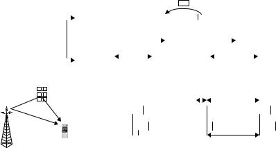
To deal with this problem and to make an OFDM signal truly insensitive to time dispersion on the radio channel, so-called cyclic-prefix insertion is typically used in case of OFDM transmission. As illustrated in Figure 4.9, cyclic-prefix insertion implies that the last part of the OFDM symbol is copied and inserted at the beginning of the OFDM symbol. Cyclic-prefix insertion thus increases the length of the OFDM symbol from Tu to Tu + TCP, where TCP is the length of the cyclic prefix, with a corresponding reduction in the OFDM symbol rate as a consequence. As illustrated in the lower part of Figure 4.9, if the correlation at the receiver side is still only carried out over a time interval Tu = 1/f , subcarrier orthogonality will then be preserved also in case of a time-dispersive channel, as long as the span of the time dispersion is shorter than the cyclic-prefix length.
In practice, cyclic-prefix insertion is carried out on the time-discrete output of the transmitter IFFT. Cyclic-prefix insertion then implies that the last NCP samples of
OFDM transmission |
53 |
the IFFT output block of length N is copied and inserted at the beginning of the block, increasing the block length from N to N + NCP. At the receiver side, the corresponding samples are discarded before OFDM demodulation by means of, for example, DFT/FFT processing.
Cyclic-prefix insertion is beneficial in the sense that it makes an OFDM signal insensitive to time dispersion as long as the span of the time dispersion does not exceed the length of the cyclic prefix. The drawback of cyclic-prefix insertion is that only a fraction Tu/(Tu + TCP) of the received signal power is actually utilized by the OFDM demodulator, implying a corresponding power loss in the demodulation. In addition to this power loss, cyclic-prefix insertion also implies a corresponding loss in terms of bandwidth as the OFDM symbol rate is reduced without a corresponding reduction in the overall signal bandwidth.
One way to reduce the relative overhead due to cyclic-prefix insertion is to reduce the subcarrier spacing f , with a corresponding increase in the symbol time Tu as a consequence. However, this will increase the sensitivity of the OFDM transmission to fast channel variations, that is high Doppler spread, as well as different types of frequency errors, see further Section 4.8.
It is also important to understand that the cyclic prefix does not necessarily have to cover the entire length of the channel time dispersion. In general, there is a trade-off between the power loss due to the cyclic prefix and the signal corruption (inter-symbol and inter-subcarrier interference) due to residual time dispersion not covered by the cyclic prefix and, at a certain point, further reduction of the signal corruption due to further increase of the cyclic-prefix length will not justify the corresponding additional power loss. This also means that, although the amount of time dispersion typically increases with the cell size, beyond a certain cell size there is often no reason to increase the cyclic prefix further as the corresponding power loss due to a further increase of the cyclic prefix would have a larger negative impact, compared to the signal corruption due to the residual time dispersion not covered by the cyclic prefix [15].
4.5 Frequency-domain model of OFDM transmission
Assuming a sufficiently large cyclic prefix, the linear convolution of a timedispersive radio channel will appear as a circular convolution during the demodulator integration interval Tu. The combination of OFDM modulation (IFFT processing), a time-dispersive radio channel, and OFDM demodulation (FFT processing) can then be seen as a frequency-domain channel as illustrated in Figure 4.10, where the frequency-domain channel taps H0, . . ., HNc−1 can be directly derived from the channel impulse response.