Encyclopedia of Sociology Vol

Assault

Robbery

Rape

Murder

Burglary

Larceny

Auto

Theft

Cleveland, William S. 1984 ‘‘Graphs in Scientific Publications.’’ American Statistician 38:261–269.

———1993 Visualizing Data. Summit N.J.: Hobart Press.

———1994 The Elements of Graphing Data, rev. ed. Summit N.J.: Hobart Press.

———, and Robert McGill 1984 ‘‘Graphical Perception: Theory, Experimentation, and Application to the Development of Graphical Methods.’’ Journal of the American Statistical Association 79:531–554.

Cook, R. Dennis 1998 Regression Graphics: Ideas for Studying Regressions through Graphics. New York: Wiley.

———, and Sanford Weisberg 1994 An Introduction to Regression Graphics. New York: Wiley.

——— 1999 Applied Regression Including Computing and Graphics. New York: Wiley.

Duncan, Otis Dudley 1961 ‘‘A Socioeconomic Index for All Occupations.’’ In Albert J. Reiss, Jr., Otis Dudley Duncan, Paul K. Hatt, and Cecil C. North, eds.,

Occupations and Social Status. New York: Free Press.

Fox, John 1991 Regression Diagnostics. Newbury Park,

Calif.: Sage.

———1997 Applied Regression Analysis, Linear Models, and Related Methods. Thousand Oaks, Calif.: Sage.

———forthcoming (a) Nonparametric Simple Regression: Scatterplot Smoothing. Thousand Oaks, Calif.: Sage.

Wainer, Howard 1997. Visual Revelations: Graphical Tales of Fate and Deception from Napoleon Bonaparte to Ross Perot. New York: Springer-Verlag.

——— forthcoming (b) Multiple and Generalized Nonparametric Regression. Thousand Oaks, Calif.: Sage.

———, and Carole Suschnigg 1989 ‘‘A Note on Gender and the Prestige of Occupations.’’ Canadian Journal of Sociology 14:353–360.

JOHN FOX

STATISTICAL INFERENCE

Funkhouser, H. Gray 1937 ‘‘Historical Development of the Graphical Representation of Statistical Data.’’ Osiris 3:267–404.

Hartigan, John A. 1975 Clustering Algorithms. New

York: Wiley.

Hastie, Trevor J., and Robert J. Tibshirani 1990 Generalized Additive Models. London: Chapman and Hall.

Huff, Darrell 1954 How to Lie with Statistics. New York: Norton.

Kruskal, Joseph B., and Myron Wish 1978 Multidimensional Scaling. Beverly Hills, Calif.: Sage.

Monette, Georges 1990 ‘‘Geometry of Multiple Regression and Interactive 3-D Graphics.’’ In John Fox and J. Scott Long, eds., Modern Methods of Data Analysis. Newbury Park, Calif.: Sage.

Ornstein, Michael D. 1976 ‘‘The Boards and Executives of the Largest Canadian Corporations: Size, Composition, and Interlocks.’’ Canadian Journal of Sociology

1:411–437.

Schmidt, Calvin F. 1983 Graphics: Design Principles and Practices. New York: Wiley.

Spence, Ian, and Stephan Lewandowsky 1990 ‘‘Graphical Perception.’’ In John Fox and J. Scott Long, eds.,

Modern Methods of Data Analysis. Newbury Park, Calif.: Sage.

Tierney, Luke 1990. Lisp-Stat: An Object-Oriented Environment for Statistical Computing and Dynamic Graphics. New York: Wiley.

Tufte, Edward R. 1983 The Visual Display of Quantitative Information. Cheshire, Conn.: Graphics Press.

———1990 Envisoning Information. Cheshire, Conn.: Graphics Press.

———1997 Visual Explanations: Images and Quantities, Evidence and Narrative. Cheshire, Conn.: Graphics Press.

Tukey, John W. 1977 Exploratory Data Analysis. Reading,

Mass.: Addison-Wesley.

Venables, W. N., and B. D. Ripley 1997 Modern Applied Statistics with S-PLUS, 2nd ed. New York: Springer-Verlag.

Making an inference involves drawing a general conclusion from specific observations. People do this every day. Upon arising in the morning, one observes that the sun is shining and that the day will be nice. The news reports the arrest of a military veteran for child abuse, and a listener infers that military veterans have special adjustment problems. Statistical inference is a way of formalizing the process of drawing general conclusions from limited information. It is a way of stating the degree of confidence one has in making an inference by using probability theory. Statistically based research allows people to move beyond speculation.

Suppose a sociologist interviews two husbands. Josh, whose wife is employed, does 50 percent of the household chores; Frank, whose wife does not work for pay, does 10 percent. Should the sociologist infer that husbands do more housework when their wives are employed? No. This difference could happen by chance with only two cases. However, what if 500 randomly selected husbands with employed wives average 50 percent of the chores and randomly selected husbands with nonemployed wives average 10 percent? Since this difference is not likely to occur by chance, the sociologist infers that husbands do more housework when their wives are employed for pay.

Researchers perform statistical inferences in three different ways. Assume that 60 percent of the respondents to a survey say they will vote for Marie Chavez. The traditional hypothesis testing approach infers that Chavez will win the election if chance processes would account for the result (60 percent support in this survey) with less than some a priori specified statistical significance level. For example, if random chance could account for the result fewer than five times in a hundred, one would say the results are statistically significant. Statistical significance levels are called the alpha

(e.g., α = .05 for the 5 percent level). If Chavez would get 60 percent support in a sample of the size selected less than 5 percent of the time by chance, one would infer that she will win. The researcher picked the 5 percent level of significance before doing the survey. (The test, including the α level, must be planned before one looks at the findings.) If one would get this result 6 percent of the time by chance, there is no inference. Note that not making the inference means just that: One does not infer that Chavez’s opponent will win.

A second strategy involves stating the likelihood of the result occurring by chance without an a priori level of significance. This strategy reports the result (60 percent of the sample supported Chavez) and the probability of getting that result by chance, say, .042. This gives readers the freedom to make their inferences using whatever level of significance they wish. Sam Jones, using the .01 level (α = .01) in the traditional approach would see that the results do not meet his criterion. He would not conclude that Chavez will win. Mara Jabar, using the .05 level, would conclude that Chavez would win.

The third strategy places a confidence interval around a result. For example, a researcher may be 95 percent confident that Chavez will get between 55 percent and 65 percent of the votes. Since the entire interval—55 percent to 65 percent—is enough for a victory, that is, is greater than 50 percent one infers that Chavez will win.

Each approach has an element of risk attached to the inference. That risk is the probability of getting the result by chance alone. Sociologists tend to pick low probabilities (e.g., .05, .01, and even .001), because they do not want to conclude that something is true when it is at all likely to have occurred by chance.

TRADITIONAL TESTS OF SIGNIFICANCE

Traditional tests of significance involve six steps. Three examples are used here to illustrate these steps: (1) A candidate will win an election, (2) mothers with at least one daughter will have different views on abortion than will mothers with only sons, and (3) the greater a person’s internal political efficacy is, the more likely that person is to vote.

Step 1: State a hypotheses (H1) in terms of statistical parameters (characteristics such as means, correlations, proportions) of the population:

H1: P(vote for the candidate) < .50. [Read: The mean for mothers with daughters is not equal to the mean for mothers with sons.]

H2: µ mothers with daughters ≠ µ mothers with sons. [Read: The means for mothers with daughters is not equal to the mean for mothers with sons.]

H3: ρ < 0.0. [Read: The popluation correlation ρ (rho) between internal political efficacy and voting is greater than zero.]

H2 says that the means are different but does not specify the direction of the difference. This is a two-tail hypothesis, meaning that it can be significant in either direction. In contrast, H1 and H2 signify the direction of the difference and are called one-tail hypotheses.

These three hypotheses are not directly testable because each involves a range of values. Step 2 states a null hypothesis, which the researcher usually wishes to reject, that has a specific value.

H10: P(vote for the candidate) = .50.

H20: µ mothers with daughters = µ mothers with sons.

H30: ρ = 0.

An important difference between one-tail and two-tail tests may have crossed the reader;s mind. Consider H10. If 40 percent of the sample supported the candidate, one fails to reject H10 because the result was in the direction opposite of that of the one-tail hypothesis. In contrast, whether mothers with daughters have a higher or lower mean attitude toward abortion than do mothers with sons, one proceeds to test H20 because a difference in either direction could be significant.

Step 3 states the a priori level of significance. Sociologists usually use the .05 level. With large samples, they sometimes use the .01 or .001 level. This paper uses the .05 level (α = .05). If the result would occur in fewer than 5 percent (corresponding to the .05 level) of the samples if the null hypothesis were true in the population, the null hypothesis is rejected in favor of the main hypothesis.

Suppose the sample correlation between internal political efficacy and voting is .56 and this would occur in fewer than 5 percent of the samples this size if the population correlation were 0 (as specified in H30). One rejects the null hypothesis, H30, and accepts the main hypothesis, H3, that the variables are correlated in the population. What if the sample correlation were .13 and a correlation this large would occur in 25 percent of the samples from a population in which the true correlation were 0? Because 25 percent exceeds the a priori significance level of 5 percent, the null hypothesis is not rejected. One cannot infer that the variables are correlated in the population. Simultaneously, the results do not prove that the population correlation is .00, simply that it could be that value.

Step 4 selects a test statistic and its critical value. Common test statistics include z, t, F, and χ2 (chi-square). The critical value is the value the test statistic must exceed to be significant at the level specified in step 3. For example, using a one-tail hypothesis, a z must exceed 1.645 to be significant at the .05 level. Using a two-tail hypothesis, a z, must exceed 1.96 to be significant at the .05 level. For t, F, and χ2, determining the critical value is more complicated because one needs to know the degrees of freedom. A formal understanding of degrees of freedom is beyond the scope of this article, but an example will give the reader an intuitive idea. If the mean of five cases is 4 and four of the cases have values of 1, 4, 5, and 2, the last case must have a value of 8 (it is the only value for the fifth case that will give a mean of 4, since 1 + 4 + 5 + 2 + x = 20, only if x = 8 and 20/5 = 4). Thus, there are n − 1 degrees of freedom. Most test statistics have different distributions for each number of degrees of freedom.

Figure 1 illustrates the z distribution. Under the z distribution, an absolute value of greater than 1.96 will occur by chance only 5 percent of the time. By chance a z > 1.96 occurs 2.5 percent of the time and a z < − 1.96 occurs 2.5 percent of the time. Thus, 1.96 is the critical z-score for a two-tail .05 level test. The critical z-score for a one-tail test at the .05 level is 1.645 or − 1.645, depending on the direction specified in the main hypothesis.

Step 5 computes the test statistic. An example appears below.

Step 6 decides whether to reject or fail to reject the null hypothesis. If the computed test statistic

exceeds the critical value, one rejects the null hypothesis and makes the inference to accept the main hypothesis. If the computed test statistic does not exceed the critical value, one fails to reject the null hypothesis and make no inference.

Example of Six Steps Applied to H1. A random sample of 200 voters shows 60 percent of them supporting the candidate. Having stated the main hypothesis (step 1) and the null hypothesis (step 2), step 3 selects an a priori significance level at α = .05, since this is the conventional level. Step 4 selects the test statistic and its critical level. To test a single percentage, a z test is used (standard textbooks on social statistics discuss how to select the appropriate tests statistics; see Agresti and Finlay 1996; Loether and McTavish 1993; Raymondo 1999; Vaughan 1997). Since the hypothesis is onetail, the critical value is 1.645 (see Figure 1).

The fifth step computes the formula for the test statistic:

z = ps − p pq

n

where ps is the proportion in the sample

p is the proportion in the population

under H 0 q is 1 − p

n is the number of people in the sample.

Thus,

The sixth step makes the decision to reject the null hypothesis, since the difference is in the predicted direction and 2.828 > 1.645. The statistical inference is that the candidate will win the election.

REPORTING THE PROBABILITY LEVEL

Many sociological researchers do not use the traditional null hypothesis model. Instead, they report the probability of the result. This way, a reader knows the probability (say, .042 or .058) rather than the significant versus not significant status. Reporting the probability level removes the ‘‘magic

Figure 1. Normal deviate (z) distribution.

of the level of significance.’’ A result that is significant at the .058 level is not categorically different from one that is significant at the .042 level. Where the traditional null hypothesis approach says that the first of these results is not significant and the second is, reporting the probability tells the reader that there is only a small difference in the degree of confidence attached to the two results. Critics of this strategy argue that the reader may adjust the significance level post hoc; that is, the reader may raise or lower the level of significance after seeing the results. It also is argued that it is the researcher, not the reader, who is the person testing the hypotheses; therefore, the researcher is responsible for selecting an a priori level of significance.

The strategy of reporting the probability is illustrated for H1. Using the tabled values or functions in standard statistical packages, the one-tail probability of a z = 2.828 is .002. The researcher reports that the candidate had 60 percent of the vote in the sample and that the probability of getting that much support by chance is .002. This provides more information than does simply saying that it is significant at the .05 level. Results that could happen only twice in 1,000 times by chance

(.002) are more compelling than are results that could happen five times in 100 (.05).

Since journal editors want to keep papers short and studies often include many tests of significance, reporting probabilities is far more efficient than going through the six-step process outlined above. The researcher must go through these steps, but the paper merely reports the probability for each test and places an asterisk along those which are significant at the .05 level. Some researchers place a single asterisk for results significant at the .05 level, two asterisks for results significant at the .01 level, and three asterisks for results significant at the .001 level.

CONFIDENCE INTERVALS

Rather than reporting the significance of a result, this approach puts a confidence interval around the result. This provides additional information in terms of the width of the confidence interval.

Using a confidence interval, a person constructs a range of values such that he or she is 95 percent confident (some use a 99 percent confi-

dence interval) that the range contains the population parameter. The confidence interval uses a two-tail approach on the assumption that the population value can be either above or below the sample value.

For the election example, H1, the confidence interval is

where z a/ 2 is the two-tail critical value for the alpha level

ps is the proportion in the sample

pis the proportion in the population

under H 0 q is 1 − p

n is the number of people in the sample

=.6 ± 1.96 × .03535

=.6 ± .0693

upper limit .669 lower limit .531

The researcher is 95 percent confident that the interval, .531 to .669, contains the true population proportion. The focus is on the confidence level (.95) for a result rather than the low likelihood of the null hypothesis (.05) used in the traditional null hypothesis testing approach.

The confidence interval has more information value than do the first two approaches. Since the value specified in the null hypothesis (H0: P = .50) is not in the confidence interval, the result is statistically significant at the .05 level. Note that a 95 percent confidence level corresponds to a .05 level of significance and that a 99 percent confidence interval corresponds to a .01 level of significance. Whenever the value specified by the null hypothesis is not in the confidence interval, the result is statistically significant. More important, the confidence interval provides an estimate of the range of possible values for the population. With 200 cases and 60 percent support, there is confidence that the candidate will win, although it may be a close election with the lower limit indicating 53.1 per-

cent of the vote or a landslide with the upper limit indicating 66.9 percent of the vote. If the sample were four times as large, n = 800, the confidence interval would be half as wide (.565–.635) and would give a better fix on the outcome.

COMPUTATION OF TESTS AND

CONFIDENCE INTERVALS

Table 1 presents formulas for some common tests of significance and their corresponding confidence intervals where appropriate. These are only a sample of the tests that are commonly used, but they cover means, differences of means, proportions, differences of proportions, contingency tables, and correlations. Not included are a variety of multivariate tests for analysis of variance, regression, path analysis, and structural equation models. The formulas shown in Table 1 are elaborated in most standard statistics textbooks (Agresti and Finlay 1996; Blalock 1979; Bohrnstedt and Knoke 1998: Loether and McTavish 1993; Raymondo 1999; Vaughan 1997).

LOGIC OF STATISTICAL INFERENCE

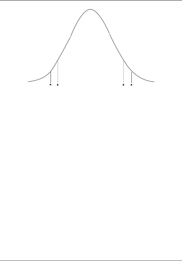
A formal treatment of the logic of statistical inference is beyond the scope of this article; the following is a simplified description. Suppose one wants to know whether a telephone survey can be thought of as a random sample. From current census information, suppose the mean, µ, income of the community is $31,800 and the standard deviation, σ, is $12,000. A graph of the complete census enumeration appears in Panel A of Figure 2. The fact that there are a few very wealthy people skews the distribution.

A telephone survey included interviews with 1,000 households. If it is random, its sample mean and standard deviation should be close to the population parameters, µ and σ, respectively. Assume that the sample has a mean of $33,200 and a standard deviation of $10,500. To distinguish these sample statistics from the population parameters, call them M and s. The sample distribution appears in Panel B by Figure 2. Note that it is similar to the population distribution but is not as smooth.

One cannot decide whether the sample could be random by looking at Panels A and B. The distributions are different, but this difference might

t with n – 1 degrees of freedom

t = M − χ s / n

z = Ps − χ PQ / N

t with n1 + n1 degrees of freedom:

where s2 =

the denominator of the t- test in the cell to the immediate left

the numerator of the z- test in the cell to the immediate left

Table 1

have occurred by chance. Statistical inference is accomplished by introducing two theoretical distributions: the sampling distribution of the mean and the z-distribution of the normal deviate. A theoretical distribution is different from the population and sample distributions in that a theoretical distribution is mathematically derived; it is not observed directly.

Sampling Distribution of the Mean. Suppose that instead of taking a single random sample of 1,000 people, one took two such samples and determined the mean of each one. With 1,000 cases, it is likely that the two samples would have means that were close together but not the same. For instance, the mean of the second sample might be $30,200. These means, $33,200 and $30,200, are pretty close to each other. For a sample to have a mean of, say $11,000, it would have to include a

greatly disproportionate share of poor families; this is not likely by chance with a random sample with n = 1,000. For a sample to have a mean of, say, $115,000, it would have to have a greatly disproportionate share of rich families. In contrast, with a sample of just two individuals, one would not be surprised if the first person had an income of $11,000 and the second had an income of $115,000.

The larger the samples are, the more stable the mean is from one sample to the next. With only 20 people in the first and second samples, the means may vary a lot, but with 100,000 people in both samples, the means should be almost identical. Mathematically, it is possible to derive a distribution of the means of all possible samples of a given n even though only a single sample is observed. It can be shown that the mean of the

Population mean is $31,800 Population standard deviation is $12,000

Sample mean is $33,200 Sample standard deviation is $10,500

sampling distribution of means is the population mean and that the standard deviation of the sampling distribution of the means is the population standard deviation divided by the square root of the sample size. The standard deviation of the mean is called the standard error of the mean:

Standard error of the mean (SEM)= σ M = σ n

This is an important derivation in statistical theory. Panel C shows the sampling distribution of the mean when the sample size is n = 1,000. It also shows the sampling distribution of the mean for n = 100. A remarkable property of the sampling distribution of the mean is that with a large sample

size, it will be normally distributed even though the population and sample distributions are skewed.

One gets a general idea of how the sample did by seeing where the sample mean falls along the sampling distribution of the mean. Using Panel C for n = 1,000, the sample M = $33,200 is a long way from the population mean. Very few samples with n = 1,000 would have means this far way from the population mean. Thus, one infers that the sample mean probably is based on a nonrandom sample.

Using the distribution in Panel C for the smaller sample size, n = 100, the sample M = $33,200 is not so unusual. With 100 cases, one should not be surprised to get a sample mean this far from the population mean.

Being able to compare the sample mean to the population mean by using the sampling distribution is remarkable, but statistical theory allows more precision. One can transform the values in the sampling distribution of the mean to a distribution of a test statistic. The appropriate test statistic is the distribution of the normal deviate, or z-distribution. It can be shown that

z = M − µ

σ/ n

If the z-value were computed for the mean of all possible samples taken at random from the population, it would be distributed as shown in Panel D of Figure 2. It will be normal, have a mean of zero, and have a variance of 1.

Where is M = $33,200 under the distribution of the normal deviate using the sample size of n = 1,000? Its z-score using the above formula is

= 33, 200 − 31, 800

z

12, 000/ 1, 000

= 3.689

Using tabled values for the normal deviate, the probability of a random sample of 1,000 cases from a population with a mean of $31,800 having a sample mean of $33,200 is less than .001. Thus, it is extremely unlikely that the sample is purely random.

With the same sample mean but with a sample of only 100 people,

= 33, 200 − 31, 800

z

12, 000/ 100

= 1.167

Using tabled values for a two-tail test, the probability of getting the sample mean this far from the population mean with a sample of 100 people is

.250. One should not infer that the sample is nonrandom, since these results could happen 25 percent of the time by chance.

The four distributions can be described for any sample statistic one wants to test (means, differences of means, proportions, differences of proportions, correlations, etc). While many of the calculations will be more complex, their logic is identical.

MULTIPLE TESTS OF SIGNIFICANCE

The logic of statistical inference applies to testing a single hypothesis. Since most studies include multiple tests, interpreting results can become extremely complex. If a researcher conducts 100 tests, 5 of them should yield results that are statistically significant at the .05 level by chance. Therefore, a study that includes many tests may find some ‘‘interesting’’ results that appear statistically significant but that really are an artifact of the number of tests conducted.

Sociologists pay less attention to ‘‘adjusting the error rate’’ than do those in most other scientific fields. A conservative approach is to divide the Type I error by the number of tests conducted. This is known as the Dunn multiple comparison test, based on the Bonferroni inequality. For example, instead of doing nine tests at the .05 level, each test is done at the .05/9 = .006 level. To be viewed as statistically significant at the .05 level, each specific test must be significant at the .006 level.

There are many specialized multiple comparison procedures, depending on whether the tests are planned before the study starts or after the results are known. Brown and Melamed (1990) describe these procedures.

POWER AND TYPE I AND TYPE II ERRORS

To this point, only one type of probability has been considered. Sociologists use statistical inference to minimize the chance of accepting a main hypothesis that is false in the population. They reject the null hypothesis only if the chances of it’s being true in the population are very small, say, α = .05. Still, by minimizing the chances of this error, sociologists increase the chance of failing to reject the null hypothesis when it should be rejected. Table 2 illustrates these two types of error.

Type I, or α, error is the probability of rejecting H0 falsely, that is, the error of deciding that H1 is right when H0 is true in the population. If one were testing whether a new program reduced drug abuse among pregnant women, the H1 would be that the program did this and the H0 would be that the program was no better than the existing one. Type I error should be minimized because it would be wrong to change programs when the new program was no better than the existing one. Type I