Encyclopedia of Sociology Vol

dents, and higher rates of literacy. One may ask whether political and economic advancement simply brings a more modern form of political violence.

One obstacle to linking high levels of terrorism with environmental factors is the problem of measuring terrorism. For the most part, this has been done by counting terrorist incidents, but international terrorism was narrowly and, more important, artificially defined to include only incidents that cause international concern, a distinction that has meant very little to the terrorists. Counting all terrorist incidents, both local and international, is better but still inadequate. Terrorist tactics, narrowly defined, represent most of what some groups, particularly those in western Europe, do but for other groups, terrorism represents only one facet of a broader armed conflict. In civil war situations, such as that in Lebanon in the 1970s, separating incidents of terrorism from the background of violence and bloodshed was futile and meaningless. And what about the extensive unquantified political and communal violence in the rural backlands of numerous third world countries? Broad statements about terrorist-prone or violence-prone societies simply cannot be made by measuring only a thin terrorist crust of that violence, if at all. The problem, however, is not merely one of counting. Although terrorists arise from the peculiarities of local situations, they may become isolated in a tiny universe of beliefs and discourse that is alien to the surrounding society. German terrorists were German, but were they Germany? In the final analysis, one is forced to dismiss the notion of a terrorist-prone society.

If terrorism cannot be explained by environmental factors, one must look into the mind of the individual terrorist for an explanation. Are there individuals who are prone to becoming terror- ists—a preterrorist personality? Encouraged by superficial similarities in the demographic profiles of terrorists—many of them have been urban middle and upper class (not economically deprived) males in their early twenties with university or at least secondary school educations—researchers searched for commmon psychological features.

Behavioral analysts painted an unappealing portrait: The composite terrorist appeared to be a

person who was narcissistic, emotionally flat, easily disillusioned, incapable of enjoyment, rigid, and a true believer who was action-oriented and risk seeking. Psychiatrists could label terrorists as neurotic and possibly sociopathic, but they found that most of them were not clinically insane. Some behavioral analysts looked for deeper connections between terrorists’ attitude toward parents and their attitudes toward authority. A few went further in claiming a physiological explanation for terrorism based on inner ear disorders, but these assertions were not given wide credence in the scientific community. The growing number of terrorists apprehended and imprisoned in the 1980s permitted more thorough studies, but while these studies occasionally unearthed tantalizing similarities, they also showed terrorists to be a diverse lot.

Much research on terrorism has been govern- ment-sponsored and therefore oriented toward the practical goal of understanding terrorism in order to defeat it. While social scientists looked for environmental or behavioral explanations for terrorism, other researchers attempted to identify terrorist vulnerabilities and successful countermeasures. They achieved a measure of success in several areas. Studies of the human dynamics of hostage situations led to the development of psychological tactics that increased the hostages’ chances of survival and a better understanding (and therefore more effective treatment) of those who had been held hostage. In some cases, specific psychological vulnerabilities were identified and exploited. With somewhat less success, researchers also examined the effects of broader policies, such as not making concessions to terrorists holding hostages and using military retaliation. The conclusion in this area were less clear-cut.

Another area of research concerned the effects of terrorism on society. Here, researchers viewed terrorism as consisting of not only the sum of terrorist actions but also the fear and alarm produced by those actions. Public opinion polls, along with measurable decisions such as not flying and avoiding certain countries, provided the measure of effect.

Some critics who are skeptical of the entire field of terrorism analysis assert that the state and

its accomplice scholars have ‘‘invented’’ terrorism as a political issue to further state agendas through manipulation of fear, the setting of public discourse, preemptive constructions of ‘‘good’’ and ‘‘evil,’’ and the creation of deliberate distractions from more serious issues. ‘‘Terrorism,’’ a pejorative term that is useful in condemning foes, has generated a lot of fear mongering, and the issue of terrorism has been harnessed to serve other agendas, but one would have to set aside the reality of terrorist campaigns to see terrorism solely as an invention of the hegemonic state. While such deconstructions reveal the ideological prejudices of their authors, they nonetheless have value in reminding other analysts to be aware of the lenses through which they view terrorism.

Over the years, research on terrorism has become more sophisticated, but in the end, terrorism confronts people with fundamental philosophical questions: Do ends justify means? How far does one go on behalf of a cause? What is the value of an individual human life? What obligations do governments have toward their own citizens if, for example, they are held hostage? Should governments or corporations ever bargain for human life? What limits can be imposed on individual liberties to ensure public safety? Is the use of military force, as a matter of choice, ever appropriate? Can assassination ever be justified? These are not matters of research. They are issues that have been dictated through the ages.

(SEE ALSO: International Law; Revolutions; Social Control;

Violent Crime; War)

REFERENCES

Barnaby, Frank 1996 Instruments of Terror. London: Satin.

Hoffman, Bruce 1998 Inside Terrorism. London: Gollancz.

Kushner, Harvey W. (ed.) 1998 The Future of Terrorism: Violence in the New Millennium. Thousand Oaks, Calif.: Sage.

Laquer, Walter 1977 Terrorism. Boston: Little Brown.

Lesser, Ian O. et al. 1999 Countering the New Terrorism. Santa Monica: Rand Corporation.

Oliverio, Annamarie 1998 The State of Terror. Albany: State University of New York Press.

O’Sullivan, Noel (ed.) 1986 Terrorism, Ideology and Revolution. Boulder, Colo: Westview.

Schmid, Alex P., and Albert J. Jongman 1988 Political Terrorism. Amsterdam: North Holland.

Simon, Jeffrey D. 1994 The Terrorist Trap: America’s Experience with Terrorism. Bloomington: Indiana University Press.

Stern, Jessica 1999 The Ultimate Terrorists. Cambridge,

Mass.: Harvard University Press.

Thackrah, John Richard 1987 Terrorism and Political Violence. London: Routledge & Kegan Paul.

Wilkinson, Paul, and Alasdair M. Stewart (eds.) 1987

Contemporary Research on Terrorism. Aberdeen, Scotland: Aberdeen University Press.

BRIAN MICHAEL JENKINS

THEOCRACY

See Religion, Politics, and War; Religious

Organizations.

TIME SERIES ANALYSIS

Longitudinal data are used commonly in sociology, and over the years sociologists have imported a wide variety of statistical procedures from other disciplines to analyze such data. Examples include survival analysis (Cox and Oakes 1984), dynamic modeling (Harvey 1990), and techniques for pooled cross-sectional and time series data (Hsiao 1986). Typically, these procedures are used to represent the causal mechanisms by which one or more outcomes are produced; a stochastic model is provided that is presumed to extract the essential means by which changes in some variables bring about changes in others (Berk 1988).

The techniques called time series analysis have somewhat different intellectual roots. Rather than try to represent explicit causal mechanisms, the goal in classical time series analysis is ‘‘simply’’ to describe some longitudinal stochastic processes in summary form. That description may be used to inform existing theory or inductively extract new

theoretical notions, but classical time series analysis does not begin with a fully articulated causal model.

However, more recent developments in time series analysis and in the analysis of longitudinal data more generally have produced a growing convergence in which the descriptive power of time series analysis has been incorporated into causal modeling and the capacity to represent certain kinds of causal mechanisms has been introduced into time series analysis (see, for example, Harvey 1990). It may be fair to say that differences between time series analysis and the causal modeling of longitudinal data are now matters of degree.

CLASSICAL TIME SERIES ANALYSIS

Classical time series analysis was developed to describe variability over time for a single unit of observation (Box and Jenkins 1976, chaps. 3 and 4). The single unit could be a person, a household, a city, a business, a market, or another entity. A popular example in sociology is the crime rate over time in a particular jurisdiction (e.g., Loftin and McDowall 1982; Chamlin 1988; Kessler and Duncan 1996). Other examples include longitudinal data on public opinion, unemployment rates, and infant mortality.

Formal Foundations. The mathematical foundations of classical time series analysis are found in difference equations. An equation ‘‘relating the values of a function y and one or more of its differences ∆y, ∆2y . . . for each x-value of some set of numbers S (for which each of these functions is defined) is called a difference equation over the set S’’ (∆y=yt−yt−1, ∆2=∆(yt−yt−1) = yt−2yt−1−yt−2, and so on) (Goldberg 1958, p. 50). The x-values specify the numbers for which the relationship holds (i.e., the domain). That is, the relationships may be true for only some values of x. In practice, the x-values are taken to be a set of successive integers that in effect indicate when a measure is taken. Then, requiring that all difference operations ∆ be taken with an interval equal to 1 (Goldberg 1958, p. 52), one gets the following kinds of results (with t replacing x): ∆2yt+kyt=2k+ 7, which can be rewritten yt−2yt−1+(1−k)yt−2= 2k+7.

Difference equations are deterministic. In practice, the social world is taken to be stochastic. Therefore, to use difference equations in time series analysis, a disturbance term is added, much as is done in conventional regression models.

ARIMA Models. Getting from stochastic difference equations to time series analysis requires that an observed time series be conceptualized as a product of an underlying substantive process. In particular, an observed time series is conceptualized as a ‘‘realization’’ of an underlying process that is assumed to be reasonably well described by an unknown stochastic difference equation (Chatfield 1996, pp. 27–28). In other words, the realization is treated as if it were a simple random sample from the distribution of all possible realizations the underlying process might produce. This is a weighty substantive assumption that cannot be made casually or as a matter of convenience. For example, if the time series is the number of lynchings by year in a southern state between 1880 and 1930, how much sense does it make to talk about observed data as a representative realization of an underlying historical process that could have produced a very large number of such realizations? Many time series are alternatively conceptualized as a population; what one sees is all there is (e.g., Freedman and Lane 1983). Then the relevance of time series analysis becomes unclear, although many of the descriptive tools can be salvaged.

If one can live with the underlying world assumed, the statistical tools time series analysis provides can be used to make inferences about which stochastic difference equation is most consistent with the data and what the values of the coefficients are likely to be. This is, of course, not much different from what is done in conventional regression analysis.

For the tools to work properly, however, one must at least assume ‘‘weak stationarity.’’ Drawing from Gottman’s didactic discussion (1981, pp. 60– 66), imagine that a very large number of realizations were actually observed and then displayed in a large two-way table with one time period in each column and one realization in each row. Weak stationarity requires that if one computed the

mean for each time period (i.e., for each column), those means would be effectively the same (and identical asymptotically). Similarly, if one computed the variance for each time period (i.e., by column), those variances would be effectively the same (and identical asymptotically). That is, the process is characterized in part by a finite mean and variance that do not change over time.

Weak stationarity also requires that the covariance of the process between periods be independent of time as well. That is, for any given lag in time (e.g., one period, two periods, or three periods), if one computed all possible covariances between columns in the table, those covariances would be effectively the same (and identical asymptotically). For example, at a lag of 2, one would compute covariances between column 1 and column 3, column 2 and column 4, column 3 and column 5, and so on. Those covariances would all be effectively the same. In summary, weak stationarity requires that the variance-covariance matrix across realizations be invariant with respect to the displacement of time. Strong stationarity implies that the joint distribution (more generally) is invariant with respect to the displacement of time. When each time period’s observations are normally distributed, weak and strong stationarity are the same. In either case, history is effectively assumed to repeat itself.

Many statistical models that are consistent with weak stationarity have been used to analyze time series data. Probably the most widely applied (and the model on which this article will focus) is associated with the work of Box and Jenkins (1976). Their most basic ARIMA (autoregressive-integrated moving-average) model has three parts: (1) an autoregressive component, (2) a moving average component, and (3) a differencing component.

Consider first the autoregressive component and yt as the variable of interest. An autoregressive

component of order p can be written as yt−

Φ1yt−1− −Φpyt−p.

Alternatively, the autoregressive component of order p (AR[p]) can be written in the form Φ (B) yy, where B is the backward shift operator—that is, (B)yt=yt−1, (B2)yt=yt−2 and so on—and φ(B)=

1−φ1B− −φpBp. For example, an autoregressive model of order 2 is yt−φ1yt−1−φ2yt−2.

A moving-average component of order q, in

contrast, can be written as εt−θ1εt−1− −θqεt−q. The variable εt is taken to be ‘‘white noise,’’ sometimes

called the ‘‘innovations process,’’ which is much like the disturbance term in regression models. It is assumed that εt is not correlated with itself and has a mean (expected value) of zero and a constant variance. It sometimes is assumed to be Gaussian as well.

The moving-average component of order q (MA[q]) also can be written in the form Θ(B)εt, where B is a backward shift operator and Θ(B) = 1 −Θ1B− −ΘqBq. For example, a moving-average model of order 2 is εt−Θ1εt−1−Θ2εt−2.

Finally, the differencing component can be written as ∆dytwhere the d is the number differences taken (or the degree of differencing). Differencing (see ‘‘Formal Foundations,’’ above) is a method to remove nonstationarity in a time series mean so that weak stationarity is achieved. It is common to see ARIMA models written in general form as Θ(B)∆dyt=Θ(B)εt.

A seasonal set of components also can be included. The set is structured in exactly the same way but uses a seasonal time reference. That is, instead of time intervals of one time period, seasonal models use time intervals such as quarters. The seasonal component usually is included multiplicatively (Box and Jenkins 1976, chap. 9; Granger and Newbold 1986, pp. 101–114; Chatfield 1996 pp. 60–61), but a discussion here is precluded by space limitations.

For many sets of longitudinal data, nonstationarity is not merely a nuisance to be removed but a finding to be highlighted. The fact that time series analysis requires stationarity does not mean that nonstationary processes are sociologically uninteresting, and it will be shown shortly that time series procedures can be combined with techniques such multiple regression when nonstationarity is an important part of the story.

ARIMA Models in Practice. In practice, one rarely knows which ARIMA model is appropriate

for the data. That is, one does not know what orders the autoregressive and moving-average components should be or what degree of differencing is required to achieve stationarity. The values of the coefficients for these models typically are unknown as well. At least three diagnostic procedures are commonly used: time series plots, the autocorrelation function, and the partial autocorrelation function.

A time series plot is simply a graph of the variable to be analyzed arrayed over time. It is always important to study time series plots carefully to get an initial sense of the data: time trends, cyclical patterns, dramatic irregularities, and outliers.

The autocorrelation function and the partial autocorrelation function of the time series are used to help specify which ARIMA model should be applied to the data (Chatfield 1996, chap. 4). The rules of thumb typically employed will be summarized after a brief illustration.

Figure 1 shows a time series plot of the simulated unemployment rate for a small city. The vertical axis is the unemployment rate, and the horizontal axis is time in quarters. There appear to be rather dramatic cycles in the data, but on closer inspection, they do not fit neatly into any simple story. For example, the cycles are not two or four periods in length (which would correspond to sixmonth or twelve-month cycles).

Figure 2 shows a plot of the autocorrelation function (ACF) of the simulated data with horizontal bands for the 95 percent confidence interval. Basically, the autocorrelation function produces a series of serial Pearson correlations for the given time series at different lags: 0, 1, 2, 3, and so on (Box and Jenkins 1976, pp. 23–36). If the series is stationary with respect to the mean, the autocorrelations should decline rapidly. If they do not, one may difference the series one or more times until the autocorrelations do decline rapidly.

For some kinds of mean nonstationarity, differencing will not solve the problem (e.g., if the nonstationarity has an exponential form). It is also important to note that mean nonstationarity may be seen in the data as differences in level for

different parts of the time series, differences in slope for different parts of the data, or even some other pattern.

In Figure 2, the autocorrelation for lag 0 is 1.0, as it should be (correlating something with itself). Thus, there are three spikes outside of the 95 percent confidence interval at lags 1, 2, and 3. Clearly, the correlations decline gradually but rather rapidly so that one may reasonably conclude that the series is already mean stationary. The gradual decline also usually is taken as a sign autoregressive processes are operating, perhaps in combination with moving-average processes and perhaps not. There also seems to be a cyclical pattern, that is consistent with the patterns in Figure 1 and usually is taken as a sign that the autoregressive process has an order of more than 1.

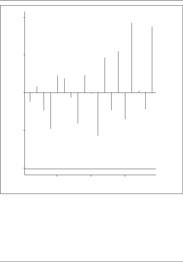
Figure 3 shows the partial autocorrelation function. The partial autocorrelation is similar to the usual partial correlation, except that what is being held constant is values of the times series at lags shorter than the lag of interest. For example, the partial autocorrelation at a lag of 4 holds constant the time series values at lags of 1, 2, and 3.

From Figure 3, it is clear that there are large spikes at lags of 1 and 2. This usually is taken to mean that the p for the autoregressive component is equal to 2. That is, an AR[2] component is necessary. In addition, the abrupt decline (rather than a rapid but gradual decline) after a lag of 2 (in this case) usually is interpreted as a sign that there is no moving-average component.

The parameters for an AR[2] model were estimated using maximum likelihood procedures. The first AR parameter estimate was 0.33, and the second was estimate -0.35. Both had t-values well in excess of conventional levels. These results are consistent with the cyclical patterns seen in Figure 1; a positive value for the first AR parameter and a negative value for the second produced the apparent cyclical patterns.

How well does the model fit? Figures 4 and 5 show, respectively, the autocorrelation function and the partial autocorrelation function for the residuals of the original time series (much like

residuals in conventional regression analysis). There are no spikes outside the 95 percent confidence interval, indicating that the residuals are probably white noise. That is, the temporal dependence in the data has been removed. One therefore can conclude that the data are consistent with an underlying autoregressive process of order 2, with

coefficients of 0.33 and -0.35. The relevance of this information will be addressed shortly.

To summarize, the diagnostics have suggested that this ARIMA model need not include any differences or a moving-average component but should include an autoregressive component of

Figure 2. Unemployment Series: Autocorrelation Function

order 2. More generally, the following diagnostic rules of thumb usually are employed, often in the order shown.

1.If the autocorrelation function does not decline rather rapidly, difference the series one or more times (perhaps up to three) until it does.

2.If either before or after differencing

the autocorrelation function declines very abruptly, a moving-average component probably is needed. The lag of the last large spike outside the confidence interval provides a good guess for the value of q. If the autocorrelation function declines rap-

idly but gradually, an autoregressive component probably is needed.

3.If the partial autocorrelation function declines very abruptly, an autoregressive component probably is needed. The lag of the last large spike outside the confidence interval provides a good guess for the value of p. If the partial autocorrelation

function declines rapidly but gradually, a moving-average component probably is needed.

4.Estimate the model’s coefficients and compute the residuals of the model. Use the rules above to examine the residuals. If there are no systematic patterns in the residuals, conclude that the model

ACF

1.0

0.8

0.6

0.4

0.2

–0.0

–0.2

Figure 4. Residuals Series: Autocorrelation Function

is consistent with the data. If there

are systematic patterns in the residuals, respecify the model and try again. Repeat until the residuals are consistent with a white noise process (i.e., no temporal dependence).

Several additional diagnostic procedures are available, but because of space limitations, they

cannot be discussed here. For an elementary discussion, see Gottman (1981), and for a more advanced discussion, see Granger and Newbold (1986).

It should be clear that the diagnostic process is heavily dependent on a number of judgment calls about which researchers could well disagree. Fortunately, such disagreements rarely matter. First, the disagreements may revolve around differences

Partial ACF

0.2

0.1

0.0

–0.1

–0.2

between models without any substantive import. There may be, for instance, no substantive consequences from reporting an MA[2] compared with an MA[3]. Second, ARIMA models often are used primarily to remove ‘‘nuisance’’ patterns in time series data (discussed below), in which case the particular model used is unimportant; it is the result that matters. Finally and more technically, if

certain assumptions are met, it is often possible to represent a low-order moving-average model as a high-order autoregressive model and a low-order autoregressive model as a high-order moving-aver- age model. Then model specification depends solely on the criteria of parsimony. That is, models with a smaller number of parameters are preferred to models with a larger number of parame-