Contents of the Experimentation Paper
Home work results.
Code combinations for each level of processor module structure.
Conclusions purpose of (the modules, their comparison with chosen analogs in function, advantages and disadvantages of the modeled realization and its analogue).
H ome work
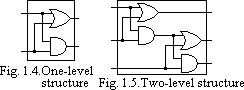
1. Define the set of logic elements to be used from the structure of each module (the structures are depicted in Fig. 1.2 and 1.3).
2. Define the function of each module.
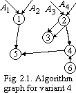
3. Define the function of each level of the module structure. The structure level is a level of logic elements which perform only one elementary logic transformation of input codes. Examples of one-level and multi-level structures are shown in Fig. 1.4 and 1.5 correspondingly.
4. Make up a procedure of defining an input binary array (x1x2x3x4x5x6) with the help of a random number generator.
5. Develop models of each module on the level of structure-functional description of each module level. Provide for possible output of code values at each structure level.
Questions for the Self-Testing
1. What is the simulation model?
 2.
Define the time characteristics (number of levels) of data
transformation in the modules being modeled.
2.
Define the time characteristics (number of levels) of data
transformation in the modules being modeled.
3. Determine the hardware expenditures in the modules of a systolic processor.
Module 2 Calculation-Graphical Work modeling of algorithmic calculation graphs using petri nets
Aim of the work: The aim of the work is to study the application of Petri nets for building computational algorithm models.
Execution of the Calculation-Graphical Work
1. Build a computational algorithm graph according to the connections between operator nodes given in Table 2.1.
2. Turn from the graph of an algorithm to a graph of a Petri net using the rules of the operator nodes illustration.
3. Build a Petri net graph.
4. Work out rules for executing the given Petri net, i.e., operating conditions of the model in performing computations.
Variants of the task are given in Table 2.1, the variant number corresponding to the student’s number in the students’ group list.
Table 2.1
Vari- Ant |
Numbers of operator nodes which are the inputs to the given one |
|||||||||||
1 |
2 |
3 |
4 |
5 |
6 |
7 |
8 |
9 |
10 |
11 |
12 |
|
1 |
Inp. |
Inp. |
7-4 |
3-3 |
2-1 |
1-6 |
3-3 |
9-6 |
6-6 |
9-9 |
9-6 |
9-7 |
2 |
Inp. |
Inp. |
1-4 |
1-6 |
3-3 |
2-3 |
6-5 |
9-6 |
7-6 |
9-6 |
7-9 |
8-7 |
3 |
Inp. |
Inp. |
2-4 |
1-1 |
4-2 |
1-3 |
2-4 |
4-5 |
6-6 |
7-8 |
3-9 |
9-8 |
4 |
Inp. |
Inp. |
2-2 |
2-6 |
1-4 |
2-5 |
1-3 |
7-6 |
6-8 |
6-7 |
6-9 |
9-9 |
5 |
Inp. |
Inp. |
1-2 |
6-7 |
2-3 |
2-7 |
4-6 |
6-6 |
6-7 |
7-7 |
7-9 |
8-6 |
6 |
Inp. |
Inp. |
4-2 |
2-2 |
2-4 |
3-2 |
1-3 |
7-4 |
7-3 |
6-9 |
6-9 |
10-9 |
7 |
Inp. |
Inp. |
1-3 |
3-4 |
4-3 |
5-2 |
6-7 |
4-2 |
6-5 |
7-9 |
4-6 |
9-9 |
8 |
Inp. |
Inp. |
2-4 |
3-1 |
4-5 |
1-3 |
5-7 |
4-5 |
7-7 |
6-8 |
8-6 |
4-3 |
9 |
Inp. |
Inp. |
5-5 |
5-6 |
3-4 |
1-3 |
1-2 |
6-5 |
7-7 |
4-2 |
4-8 |
10-9 |
10 |
Inp. |
Inp. |
1-2 |
4-2 |
6-7 |
2-2 |
3-1 |
4-4 |
5-8 |
4-2 |
5-6 |
8-7 |
11 |
Inp. |
Inp. |
2-2 |
7-2 |
7-4 |
5-1 |
4-4 |
6-3 |
4-7 |
8-9 |
10-9 |
4-2 |
12 |
Inp. |
Inp. |
4-5 |
3-3 |
6-2 |
8-1 |
9-4 |
2-6 |
5-7 |
5-9 |
6-5 |
9-7 |
13 |
Inp. |
Inp. |
5-2 |
5-7 |
6-2 |
4-4 |
3-9 |
4-5 |
6-8 |
9-11 |
1-4 |
6-7 |
14 |
Inp. |
Inp. |
4-6 |
6-7 |
1-2 |
3-4 |
4-5 |
5-6 |
6-7 |
7-8 |
8-9 |
9-10 |
15 |
Inp. |
Inp. |
11-1 |
7-5 |
6-5 |
3-2 |
4-4 |
9-1 |
5-8 |
3-11 |
4-7 |
4-9 |
Table 2.1 (Continued)
Vari- ant |
Numbers of operator nodes which are the inputs to the given one |
|||||||||||
1 |
2 |
3 |
4 |
5 |
6 |
7 |
8 |
9 |
10 |
11 |
12 |
|
16 |
Inp. |
Inp. |
1-5 |
8-2 |
3-3 |
5-3 |
5-3 |
5-1 |
11-6 |
5-2 |
7-9 |
2-4 |
17 |
Inp. |
Inp. |
1-1 |
6-5 |
3-4 |
5-12 |
3-4 |
7-9 |
4-4 |
6-6 |
2-4 |
11-8 |
18 |
Inp. |
Inp. |
4-2 |
2-5 |
2-1 |
11-4 |
5-6 |
6-7 |
6-7 |
4-2 |
9-6 |
10-3 |
19 |
Inp. |
Inp. |
12-5 |
12-1 |
2-3 |
7-2 |
4-3 |
4-8 |
5-8 |
9-7 |
5-5 |
2-5 |
20 |
Inp. |
Inp. |
11-1 |
12-2 |
4-6 |
3-5 |
6-4 |
6-6 |
7-6 |
4-6 |
3-5 |
3-5 |
21 |
Inp. |
Inp. |
4-2 |
3-3 |
4-2 |
3-7 |
4-6 |
5-5 |
7-4 |
8-3 |
9-2 |
10-1 |
22 |
Inp. |
Inp. |
5-5 |
6-6 |
7-7 |
8-8 |
6-5 |
7-2 |
8-7 |
7-4 |
10-2 |
11-1 |
23 |
Inp. |
Inp. |
6-7 |
7-7 |
8-8 |
8-9 |
4-4 |
3-3 |
6-9 |
11-3 |
10-1 |
11-4 |
24 |
Inp. |
Inp. |
4-5 |
6-2 |
4-6 |
3-1 |
4-2 |
7-2 |
3-3 |
4-4 |
5-5 |
3-7 |
25 |
Inp. |
Inp. |
1-1 |
6-5 |
3-4 |
5-12 |
3-4 |
7-9 |
4-4 |
6-6 |
2-4 |
11-7 |
26 |
Inp. |
Inp. |
2-4 |
1-1 |
4-2 |
1-3 |
2-4 |
4-5 |
6-6 |
7-8 |
3-8 |
8-7 |
27 |
Inp. |
Inp. |
1-2 |
6-7 |
2-3 |
2-7 |
4-6 |
6-7 |
6-7 |
7-7 |
7-9 |
9-6 |
28 |
Inp. |
Inp. |
2-2 |
7-2 |
7-4 |
5-1 |
4-4 |
6-4 |
4-7 |
8-9 |
10-9 |
4-3 |
29 |
Inp. |
Inp. |
1-5 |
6-2 |
3-3 |
5-4 |
5-3 |
5-1 |
11-6 |
5-2 |
7-9 |
3-4 |
30 |
Inp. |
Inp. |
4-5 |
6-2 |
4-5 |
3-1 |
4-2 |
7-2 |
3-3 |
3-4 |
5-5 |
2-7 |
 Example.
Let us build a part of the algorithm graph for variant 4. The first
five operator nodes are connected with each other in the way shown in
Fig. 2.1.
Example.
Let us build a part of the algorithm graph for variant 4. The first
five operator nodes are connected with each other in the way shown in
Fig. 2.1.
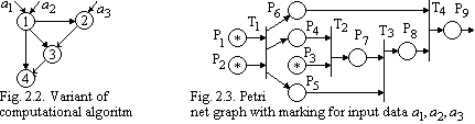
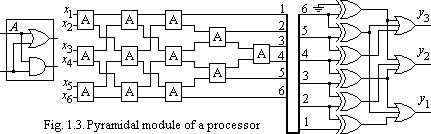
We build a Petri net on the basis of the algorithm in the following way. Let the computational algorithm be as shown in Fig. 2.2.
According to the rules of building Petri nets, an arc is replaced by a position and an operator node is replaced by a transition. Using these rules we get a Petri net graph shown in Fig. 2.3.