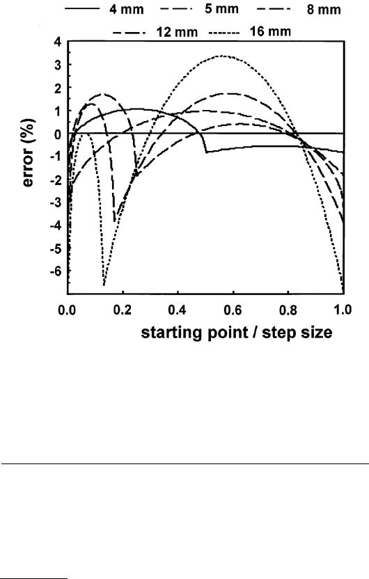
FIGURE 13.7 The errors in surface estimates by numerical integration for different step sizes h presented as percentage of the exact solution, as a function of the position of the first section, located between 0 and h. (From R. G. Aarnink et al., Physiol. Meas., 16, 141-150, 1995. With permission.)

error in volume estimation is less than 5%. Although clinical application might introduce additional errors such as movement artifacts, this rule provides a good indication of the intersection distance that should be used for good approximations with numerical integration.

13.3 Indicator Dilution Methods

The principle of the indicator dilution theory to determine gas or fluid volume was originally developed by Stewart and Hamilton. It is based on the following concept: if the concentration of an indicator that is uniformly dispersed in an unknown volume is determined, and the volume of the indicator is known, the unknown volume can be determined. Assuming a single in-flow and single out-flow model, all input will eventually emerge through the output channel, and the volumetric flow rate can be used to identify the volume flow. It can be described with two equations, of which the second is used to determine the volume using the result of the first equation [16]:

© 1999 by CRC Press LLC

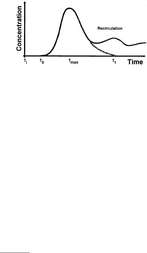
FIGURE 13.8 The time-concentration curve of the indicator is used to obtain the unknown volume of the fluid. The area under the time-concentration curve is needed to estimate the volumetric flow rate, and this flow rate can be used to estimate the volume flow. For accurate determination of the flow rate, it is necessary to extrapolate the first pass response before the area under the curve is estimated.

The integrated value of the concentration over time can be obtained from the concentration-time curve (Figure 13.8) using planimetry and an approximation described by the Riemann sum expression (Equation 13.13). Care must be taken to remove the influence of the effect of recirculation of the indicator. An indicator is suitable for use in the dilution method if it can be detected and measured, and remains within the circulation during at least its first circuit, without doing harm to the object. Subsequent removal from the circulation is an advantage. Dyes such as Coomassie blue and indocyanine green were initially used, using the peak spectral absorption at certain wavelengths to detect the indicator. Also, radioisotopes such as I-labeled human serum albumin have been used. Currently, the use of cooled saline has become routine in measurement of cardiac output in the intensive care unit.

Thermodilution

To perform cardiac output measurements, a cold bolus (with a temperature gradient of at least 10E) is injected into the right atrium and the resulting change in temperature of the blood in the pulmonary artery is detected using a rapidly responding thermistor. After recording the temperature-time curve, the blood flow is calculated using a modified Stewart-Hamilton equation. This equation can be described as follows [17]:

© 1999 by CRC Press LLC

The terms on the left represent the cooling of the blood (with temperature Tb), as caused by the injection of a cold bolus with volume Vi , with temperature Ti , specific weight SWi and specific heat SHi. The same amount of “indicator” must appear in the blood (with specific weight and heat SWb and SHb, respectively) downstream to the point of injection, where it is detected in terms of the time-course of the temperature Tb in the flow F by means of a thermistor. The flow can be described as:

where K (the so-called calculation constant) is described as:

This constant is introduced to the computer by the user. Ti is usually measured at the proximal end of the injection line; therefore, a “correction factor” C must be introduced to correct for the estimated losses of cold saline in the catheter, due to the dead space volume. Furthermore, the warming effect of the injected fluid during passing through the blood must be corrected; this warming effect depends on the speed of injection, the length of immersion of the catheter, and the temperature gradient. This warming effect reduces the actual amount of injected fluid, so the correction factor C is less than 1 [17].

Radionuclide Techniques

Radionuclide imaging is a common noninvasive technique used in the evaluation of cardiac function and disease. It can be compared to X-ray radiology, but now the radiation emanating from inside the human body is used to construct the image. Radionuclide imaging has proven useful to obtain ejection fraction and left ventricular volume. As in thermodilution, a small volume of indicator is injected peripherally; in this case, radioisotopes (normally indicated as radiopharmaceuticals) are used. The radioactive decay of radioisotopes leads to the emission of alpha, beta, gamma, and X radiation, depending on the radionuclide used. For in vivo imaging, only gammaor X-radiation can be detected with detectors external to the body, while the minimal amount of energy of the emitted photons should be greater than 50 keV. Using a photon counter such as a Gamma camera, equipped with a collimator, the radioactivity can be recorded. Two techniques are commonly used: the first pass method and the dynamic recording method [11].

First Pass Method

To inject a radionuclide bolus into the blood system, a catheter is inserted in a vein, for example, an external jugular or an antecubital vein. The camera used to detect the radioactive bolus is usually positioned in the left anterior oblique position to obtain optimal right and left ventricular separation, and is tilted slightly in an attempt to separate left atrial activity from that of the left ventricle. First, the background radiation is obtained by counting the background emissions. Then, a region of interest is determined over the left ventricle and a time-activity curve is generated by counting the photon emissions over time. The radioactivity count over time usually reveals peaks at different moments; the first peak occurs when the radioactivity in the right ventricle is counted, the second peak is attributed to left ventricular activity. More peaks can occur during recirculation of the radioactivity. After correction for

© 1999 by CRC Press LLC