Before we can begin to develop an understanding of the static and time changing characteristics of measurements, it is necessary to build a framework for understanding the process involved, setting down the main words used to describe concepts as we progress.

Measurement is the process by which relevant information about a system of interest is interpreted using the human thinking ability to define what is believed to be the new knowledge gained. This information may be obtained for purposes of controlling the behavior of the system (as in engineering applications) or for learning more about it (as in scientific investigations).

The basic entity needed to develop the knowledge is called data, and it is obtained with physical assemblies known as sensors that are used to observe or sense system variables. The terms information and knowledge tend to be used interchangeably to describe the entity resulting after data from one or more sensors have been processed to give more meaningful understanding. The individual variables being sensed are called measurands.

The most obvious way to make observations is to use the human senses of seeing, feeling, and hearing. This is often quite adequate or may be the only means possible. In many cases, however, sensors are used that have been devised by man to enhance or replace our natural sensors. The number and variety of sensors is very large indeed. Examples of man-made sensors are those used to measure temperature, pressure, or length. The process of sensing is often called transduction, being made with transducers. These man-made sensor assemblies, when coupled with the means to process the data into knowledge, are generally known as (measuring) instrumentation.

The degree of perfection of a measurement can only be determined if the goal of the measurement can be defined without error. Furthermore, instrumentation cannot be made to operate perfectly. Because of these two reasons alone, measuring instrumentation cannot give ideal sensing performance and it must be selected to suit the allowable error in a given situation.

© 1999 by CRC Press LLC

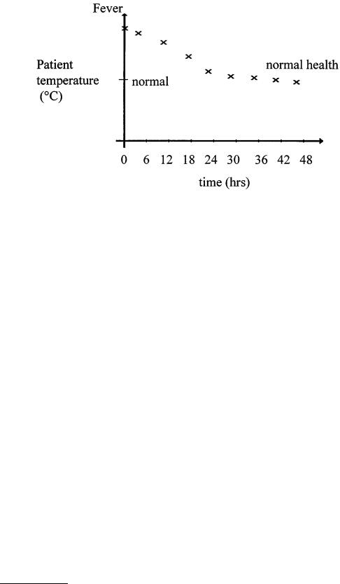
FIGURE 3.1 A patient’s temperature chart shows changes taking place over time.

Measurement is a process of mapping actually occurring variables into equivalent values. Deviations from perfect measurement mappings are called errors: what we get as the result of measurement is not exactly what is being measured. A certain amount of error is allowable provided it is below the level of uncertainty we can accept in a given situation. As an example, consider two different needs to measure the measurand, time. The uncertainty to which we must measure it for daily purposes of attending a meeting is around a 1 min in 24 h. In orbiting satellite control, the time uncertainty needed must be as small as milliseconds in years. Instrumentation used for the former case costs a few dollars and is the watch we wear; the latter instrumentation costs thousands of dollars and is the size of a suitcase.

We often record measurand values as though they are constant entities, but they usually change in value as time passes. These “dynamic” variations will occur either as changes in the measurand itself or where the measuring instrumentation takes time to follow the changes in the measurand — in which case it may introduce unacceptable error.

For example, when a fever thermometer is used to measure a person’s body temperature, we are looking to see if the person is at the normally expected value and, if it is not, to then look for changes over time as an indicator of his or her health. Figure 3.1 shows a chart of a patient’s temperature. Obviously, if the thermometer gives errors in its use, wrong conclusions could be drawn. It could be in error due to incorrect calibration of the thermometer or because no allowance for the dynamic response of the thermometer itself was made.

Instrumentation, therefore, will only give adequately correct information if we understand the static and dynamic characteristics of both the measurand and the instrumentation. This, in turn, allows us to then decide if the error arising is small enough to accept.

As an example, consider the electronic signal amplifier in a sound system. It will be commonly quoted as having an amplification constant after feedback if applied to the basic amplifier of, say, 10. The actual amplification value is dependent on the frequency of the input signal, usually falling off as the frequency increases. The frequency response of the basic amplifier, before it is configured with feedback that markedly alters the response and lowers the amplification to get a stable operation, is shown as a graph of amplification gain versus input frequency. An example of the open loop gain of the basic amplifier is given in Figure 3.2. This lack of uniform gain over the frequency range results in error — the sound output is not a true enough representation of the input.

© 1999 by CRC Press LLC

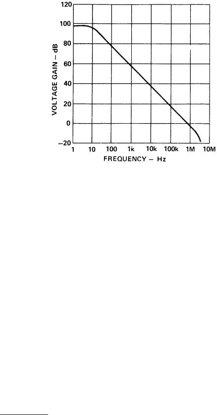
FIGURE 3.2 This graph shows how the amplification of an amplifier changes with input frequency.

Before we can delve more deeply into the static and dynamic characteristics of instrumentation, it is necessary to understand the difference in meaning between several basic terms used to describe the results of a measurement activity.

The correct terms to use are set down in documents called standards. Several standardized metrology terminologies exist but they are not consistent. It will be found that books on instrumentation and statements of instrument performance often use terms in different ways. Users of measurement information need to be constantly diligent in making sure that the statements made are interpreted correctly.

The three companion concepts about a measurement that need to be well understood are its discrimination, its precision, and its accuracy. These are too often used interchangeably — which is quite wrong to do because they cover quite different concepts, as will now be explained.

When making a measurement, the smallest increment that can be discerned is called the discrimination. (Although now officially declared as wrong to use, the term resolution still finds its way into books and reports as meaning discrimination.) The discrimination of a measurement is important to know because it tells if the sensing process is able to sense fine enough changes of the measurand.

Even if the discrimination is satisfactory, the value obtained from a repeated measurement will rarely give exactly the same value each time the same measurement is made under conditions of constant value of measurand. This is because errors arise in real systems. The spread of values obtained indicates the precision of the set of the measurements. The word precision is not a word describing a quality of the measurement and is incorrectly used as such. Two terms that should be used here are: repeatability, which describes the variation for a set of measurements made in a very short period; and the reproducibility, which is the same concept but now used for measurements made over a long period. As these terms describe the outcome of a set of values, there is need to be able to quote a single value to describe the overall result of the set. This is done using statistical methods that provide for calculation of the “mean value” of the set and the associated spread of values, called its variance.

The accuracy of a measurement is covered in more depth elsewhere so only an introduction to it is required here. Accuracy is the closeness of a measurement to the value defined to be the true value. This

© 1999 by CRC Press LLC

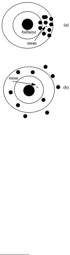
FIGURE 3.3 Two sets of arrow shots fired into a target allow understanding of the measurement concepts of discrimination, precision, and accuracy. (a) The target used for shooting arrows allows investigation of the terms used to describe the measurement result. (b) A different set of placements.

concept will become clearer when the following illustrative example is studied for it brings together the three terms into a single perspective of a typical measurement.

Consider then the situation of scoring an archer shooting arrows into a target as shown in Figure 3.3(a). The target has a central point — the bulls-eye. The objective for a perfect result is to get all arrows into the bulls-eye. The rings around the bulls-eye allow us to set up numeric measures of less-perfect shooting performance.

Discrimination is the distance at which we can just distinguish (i.e., discriminate) the placement of one arrow from another when they are very close. For an arrow, it is the thickness of the hole that decides the discrimination. Two close-by positions of the two arrows in Figure 3.3(a) cannot be separated easily. Use of thinner arrows would allow finer detail to be decided.

Repeatability is determined by measuring the spread of values of a set of arrows fired into the target over a short period. The smaller the spread, the more precise is the shooter. The shooter in Figure 3.3(a) is more precise than the shooter in Figure 3.3(b).

If the shooter returned to shoot each day over a long period, the results may not be the same each time for a shoot made over a short period. The mean and variance of the values are now called the reproducibility of the archer’s performance.

Accuracy remains to be explained. This number describes how well the mean (the average) value of the shots sits with respect to the bulls-eye position. The set in Figure 3.3(b) is more accurate than the set in Figure 3.3(a) because the mean is nearer the bulls-eye (but less precise!).

At first sight, it might seem that the three concepts of discrimination, precision, and accuracy have a strict relationship in that a better measurement is always that with all three aspects made as high as is affordable. This is not so. They need to be set up to suit the needs of the application.

We are now in a position to explore the commonly met terms used to describe aspects of the static and the dynamic performance of measuring instrumentation.

© 1999 by CRC Press LLC

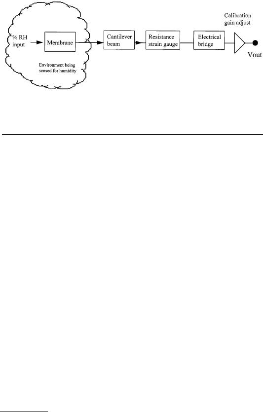
FIGURE 3.4 Instruments are formed from a connection of blocks. Each block can be represented by a conceptual and mathematical model. This example is of one type of humidity sensor.

3.1 Static Characteristics of Instrument Systems

Output/Input Relationship

Instrument systems are usually built up from a serial linkage of distinguishable building blocks. The actual physical assembly may not appear to be so but it can be broken down into a representative diagram of connected blocks. Figure 3.4 shows the block diagram representation of a humidity sensor. The sensor is activated by an input physical parameter and provides an output signal to the next block that processes the signal into a more appropriate state.

A key generic entity is, therefore, the relationship between the input and output of the block. As was pointed out earlier, all signals have a time characteristic, so we must consider the behavior of a block in terms of both the static and dynamic states.

The behavior of the static regime alone and the combined static and dynamic regime can be found through use of an appropriate mathematical model of each block. The mathematical description of system responses is easy to set up and use if the elements all act as linear systems and where addition of signals can be carried out in a linear additive manner. If nonlinearity exists in elements, then it becomes considerably more difficult — perhaps even quite impractical — to provide an easy to follow mathematical explanation. Fortunately, general description of instrument systems responses can be usually be adequately covered using the linear treatment.

The output/input ratio of the whole cascaded chain of blocks 1, 2, 3, etc. is given as:

[output/input]total = [output/input]1 × [output/input]2 × [output/input]3 …

The output/input ratio of a block that includes both the static and dynamic characteristics is called the transfer function and is given the symbol G.

The equation for G can be written as two parts multiplied together. One expresses the static behavior of the block, that is, the value it has after all transient (time varying) effects have settled to their final state. The other part tells us how that value responds when the block is in its dynamic state. The static part is known as the transfer characteristic and is often all that is needed to be known for block description.

The static and dynamic response of the cascade of blocks is simply the multiplication of all individual blocks. As each block has its own part for the static and dynamic behavior, the cascade equations can be rearranged to separate the static from the dynamic parts and then by multiplying the static set and the dynamic set we get the overall response in the static and dynamic states. This is shown by the sequence of Equations 3.1 to 3.4.

© 1999 by CRC Press LLC

An example will clarify this. A mercury-in-glass fever thermometer is placed in a patient’s mouth. The indication slowly rises along the glass tube to reach the final value, the body temperature of the person. The slow rise seen in the indication is due to the time it takes for the mercury to heat up and expand up the tube. The static sensitivity will be expressed as so many scale divisions per degree and is all that is of interest in this application. The dynamic characteristic will be a time varying function that settles to unity after the transient effects have settled. This is merely an annoyance in this application but has to be allowed by waiting long enough before taking a reading. The wrong value will be viewed if taken before the transient has settled.

At this stage, we will now consider only the nature of the static characteristics of a chain; dynamic response is examined later.

If a sensor is the first stage of the chain, the static value of the gain for that stage is called the sensitivity. Where a sensor is not at the input, it is called the amplification factor or gain. It can take a value less than unity where it is then called the attenuation.

Sometimes, the instantaneous value of the signal is rapidly changing, yet the measurement aspect part is static. This arises when using ac signals in some forms of instrumentation where the amplitude of the waveform, not its frequency, is of interest. Here, the static value is referred to as its steady state transfer characteristic.

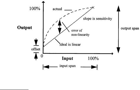
Sensitivity may be found from a plot of the input and output signals, wherein it is the slope of the graph. Such a graph, see Figure 3.5, tells much about the static behavior of the block.

The intercept value on the y-axis is the offset value being the output when the input is set to zero. Offset is not usually a desired situation and is seen as an error quantity. Where it is deliberately set up, it is called the bias.

The range on the x-axis, from zero to a safe maximum for use, is called the range or span and is often expressed as the zone between the 0% and 100% points. The ratio of the span that the output will cover

FIGURE 3.5 The graph relating input to output variables for an instrument block shows several distinctive static performance characteristics.

© 1999 by CRC Press LLC

FIGURE 3.6 Drift in the performance of an instrument takes many forms: (a) drift over time for a spring balance; (b) how an electronic amplifier might settle over time to a final value after power is supplied; (c) drift, due to temperature, of an electronic amplifier varies with the actual temperature of operation.

for the related input range is known as the dynamic range. This can be a confusing term because it does not describe dynamic time behavior. It is particularly useful when describing the capability of such instruments as flow rate sensors — a simple orifice plate type may only be able to handle dynamic ranges of 3 to 4, whereas the laser Doppler method covers as much as 107 variation.

Drift

It is now necessary to consider a major problem of instrument performance called instrument drift. This is caused by variations taking place in the parts of the instrumentation over time. Prime sources occur as chemical structural changes and changing mechanical stresses. Drift is a complex phenomenon for which the observed effects are that the sensitivity and offset values vary. It also can alter the accuracy of the instrument differently at the various amplitudes of the signal present.

Detailed description of drift is not at all easy but it is possible to work satisfactorily with simplified values that give the average of a set of observations, this usually being quoted in a conservative manner. The first graph (a) in Figure 3.6 shows typical steady drift of a measuring spring component of a weighing balance. Figure 3.6(b) shows how an electronic amplifier might settle down after being turned on.

Drift is also caused by variations in environmental parameters such as temperature, pressure, and humidity that operate on the components. These are known as influence parameters. An example is the change of the resistance of an electrical resistor, this resistor forming the critical part of an electronic amplifier that sets its gain as its operating temperature changes.

Unfortunately, the observed effects of influence parameter induced drift often are the same as for time varying drift. Appropriate testing of blocks such as electronic amplifiers does allow the two to be separated to some extent. For example, altering only the temperature of the amplifier over a short period will quickly show its temperature dependence.

Drift due to influence parameters is graphed in much the same way as for time drift. Figure 3.6(c) shows the drift of an amplifier as temperature varies. Note that it depends significantly on the temperature

© 1999 by CRC Press LLC

of operation, implying that the best designs are built to operate at temperatures where the effect is minimum.

Careful consideration of the time and influence parameter causes of drift shows they are interrelated and often impossible to separate. Instrument designers are usually able to allow for these effects, but the cost of doing this rises sharply as the error level that can be tolerated is reduced.

Hysteresis and Backlash

Careful observation of the output/input relationship of a block will sometimes reveal different results as the signals vary in direction of the movement. Mechanical systems will often show a small difference in length as the direction of the applied force is reversed. The same effect arises as a magnetic field is reversed in a magnetic material. This characteristic is called hysteresis. Figure 3.7 is a generalized plot of the output/input relationship showing that a closed loop occurs. The effect usually gets smaller as the amplitude of successive excursions is reduced, this being one way to tolerate the effect. It is present in most materials. Special materials have been developed that exhibit low hysteresis for their application — transformer iron laminations and clock spring wire being examples.

Where this is caused by a mechanism that gives a sharp change, such as caused by the looseness of a joint in a mechanical joint, it is easy to detect and is known as backlash.

Saturation

So far, the discussion has been limited to signal levels that lie within acceptable ranges of amplitude. Real system blocks will sometimes have input signal levels that are larger than allowed. Here, the dominant errors that arise — saturation and crossover distortion — are investigated.

As mentioned above, the information bearing property of the signal can be carried as the instantaneous value of the signal or be carried as some characteristic of a rapidly varying ac signal. If the signal form is not amplified faithfully, the output will not have the same linearity and characteristics.

The gain of a block will usually fall off with increasing size of signal amplitude. A varying amplitude input signal, such as the steadily rising linear signal shown in Figure 3.8, will be amplified differently according to the gain/amplitude curve of the block. In uncompensated electronic amplifiers, the larger amplitudes are usually less amplified than at the median points.

At very low levels of input signal, two unwanted effects may arise. The first is that small signals are often amplified more than at the median levels. The second error characteristic arises in electronic amplifiers because the semiconductor elements possess a dead-zone in which no output occurs until a small threshold is exceeded. This effect causes crossover distortion in amplifiers.

If the signal is an ac waveform, see Figure 3.9, then the different levels of a cycle of the signal may not all be amplified equally. Figure 3.9(a) shows what occurs because the basic electronic amplifying elements are only able to amplify one polarity of signal. The signal is said to be rectified. Figure 3.9(b) shows the effect when the signal is too large and the top is not amplified. This is called saturation or clipping. (As with many physical effects, this effect is sometimes deliberately invoked in circuitry, an example being where it is used as a simple means to convert sine-waveform signals into a square waveform.) Crossover distortion is evident in Figure 3.9(c) as the signal passes from negative to positive polarity.

Where input signals are small, such as in sensitive sensor use, the form of analysis called small signal behavior is needed to reveal distortions. If the signals are comparatively large, as for digital signal considerations, a large signal analysis is used. Design difficulties arise when signals cover a wide dynamic range because it is not easy to allow for all of the various effects in a single design.

Bias

Sometimes, the electronic signal processing situation calls for the input signal to be processed at a higher average voltage or current than arises normally. Here a dc value is added to the input signal to raise the level to a higher state as shown in Figure 3.10. A need for this is met where only one polarity of signal

© 1999 by CRC Press LLC