To properly appreciate instrumentation design and its use, it is now necessary to develop insight into the most commonly encountered types of dynamic response and to develop the mathematical modeling basis that allows us to make concise statements about responses.

If the transfer relationship for a block follows linear laws of performance, then a generic mathematical method of dynamic description can be used. Unfortunately, simple mathematical methods have not been found that can describe all types of instrument responses in a simplistic and uniform manner. If the behavior is nonlinear, then description with mathematical models becomes very difficult and might be impracticable. The behavior of nonlinear systems can, however, be studied as segments of linear behavior joined end to end. Here, digital computers are effectively used to model systems of any kind provided the user is prepared to spend time setting up an adequate model.

Now the mathematics used to describe linear dynamic systems can be introduced. This gives valuable insight into the expected behavior of instrumentation, and it is usually found that the response can be approximated as linear.

The modeled response at the output of a block Gresult is obtained by multiplying the mathematical expression for the input signal Ginput by the transfer function of the block under investigation Gresponse , as shown in Equation 3.5.

To proceed, one needs to understand commonly encountered input functions and the various types of block characteristics. We begin with the former set: the so-called forcing functions.

Forcing Functions

Let us first develop an understanding of the various types of input signal used to perform tests. The most commonly used signals are shown in Figure 3.12. These each possess different valuable test features. For example, the sine-wave is the basis of analysis of all complex wave-shapes because they can be formed as a combination of various sine-waves, each having individual responses that add to give all other waveshapes. The step function has intuitively obvious uses because input transients of this kind are commonly encountered. The ramp test function is used to present a more realistic input for those systems where it is not possible to obtain instantaneous step input changes, such as attempting to move a large mass by a limited size of force. Forcing functions are also chosen because they can be easily described by a simple mathematical expression, thus making mathematical analysis relatively straightforward.

Characteristic Equation Development

The behavior of a block that exhibits linear behavior is mathematically represented in the general form of expression given as Equation 3.6.

Here, the coefficients a2, a1, and a0 are constants dependent on the particular block of interest. The lefthand side of the equation is known as the characteristic equation. It is specific to the internal properties of the block and is not altered by the way the block is used.

The specific combination of forcing function input and block characteristic equation collectively decides the combined output response. Connections around the block, such as feedback from the output to the input, can alter the overall behavior significantly: such systems, however, are not dealt with in this section being in the domain of feedback control systems.

Solution of the combined behavior is obtained using Laplace transform methods to obtain the output responses in the time or the complex frequency domain. These mathematical methods might not be familiar to the reader, but this is not a serious difficulty for the cases most encountered in practice are

© 1999 by CRC Press LLC

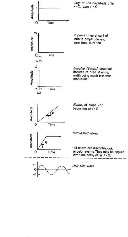
FIGURE 3.12 The dynamic response of a block can be investigated using a range of simple input forcing functions. (From P. H. Sydenham, Handbook of Measurement Science, Vol. 2, Chichester, U.K., John Wiley & Sons, 1983. With permission.)

well documented in terms that are easily comprehended, the mathematical process having been performed to yield results that can be used without the same level of mathematical ability. More depth of explanation can be obtained from [1] or any one of the many texts on energy systems analysis. Space here only allows an introduction; this account is linked to [1], Chapter 17, to allow the reader to access a fuller description where needed.

© 1999 by CRC Press LLC