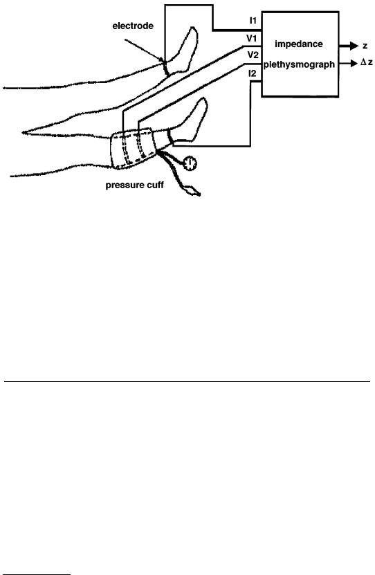
FIGURE 13.2 Electrode positioning for impedance plethysmography used for early detection of peripheral atherosclerosis: the outer two supply current while the inner two measure voltage. The combination of these two is used to obtain the changes in impedance, and these changes are then used to obtain the changes in volume of the leg. (From R. Shankar and J. G. Webster, IEEE Trans. Biomed. Eng., 38, 62-67, 1993. With permission.)

with VRC and VAB the contributions of the rib cage (RC) and abdominal compartments (AB) to the tidal volume VT. Calibration can be performed by determining the calibration constant in an isovolume measurement or by regression methods of differences in inductance changes due to a different body position or a different state of sleep [10]. Once it is calibrated, the respiratory inductive plethysmograph can be used for noninvasive monitoring of changes of thoracic volume and respiratory patterns.

13.2 Numerical Integration with Imaging

For diagnostic purposes in health care, a number of imaging modalities are currently in use (see also Chapter 79 on medical imaging). Webb nicely reviewed the scientific basis and physical principles of medical imaging [11].

With medical imaging modalities, diameters of objects can be determined in a noninvasive manner. By applying these diameters in an appropriate formula for volume calculation, the size of the object can be estimated. For example, in a clinical setting, the prostate volume Vp can be approximated with an ellipsoid volume calculation:

with H the height, W the width, and L the length of the prostate as illustrated in Figure 13.4. Variations have been introduced to find the best formulae to estimate the prostate volume [12, 13]. Also, for the determination of ventricular volumes, formulae have been derived, based on the following variation of

© 1999 by CRC Press LLC

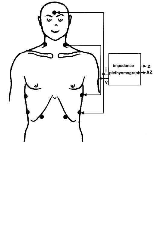
FIGURE 13.3 A second example of electrode positioning for impedance plethysmography, here used to estimate stroke volume: the outer two supply current while the inner two measure voltage. (From N. Verschoor et al., Physiol. Meas., 17, 29-35, 1996. With permission.)

the formula for prostate volume measurements: (1) the volume is obtained with the same formula as for prostate volume measurements, (2) the two short axes are equal, (3) the long axis is twice the short axis, and (4) the internal diameter is used for all axes.

By displaying cross-sectional images of a 3-D object (e.g., an organ), volume calculations can also be performed by integrating areas of the organ over a sequence of medical images as illustrated in Figure 13.5. For ultrasound images, applications have been reported in the literature on prostate, heart, bladder, and kidney volume. The application of integration techniques involves the application of segmentation algorithms on sequences of images, either in transverse direction with fixed intersection distance or in the radial with images at a fixed intersection angle.

For a volume defined by the function f(x,y,z), the volume can be calculated from:

x=x1 y=y1 z=z1

© 1999 by CRC Press LLC

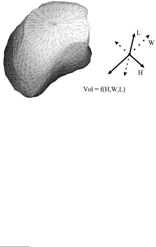
FIGURE 13.4 Volume estimate of a prostate, obtained from 3-D reconstruction of cross-sectional images, using the dimensions in three planes: the length, height, and width in a volume formula describing an ellipsoid shape.

By applying numerical integration, the volume calculation using an integral is approximated by a linear combination of the values of the integrand. For reasons of simplicity, this approximation is first illustrated for a one-dimensional case:

x=a

In this equation, x1, x2, …, xn are n points chosen in the interval of integration [a,b], and the numbers w1, w2, …, wn are n weights corresponding to these points. This approximation can also be expressed in the so-called Riemann sum:

For volume calculation, the Riemann sum needs to be extended to a three-dimensional case:

x=x1 y=y1 z=z1

This three-dimensional case can be reduced by assuming that (xi+1 – xi)(yi+1 – yi) f(pijk) represents the surface Sk of a two-dimensional section at position zk , while (zk+1 – zk) is constant for every k and equals h, the intersection distance:

© 1999 by CRC Press LLC

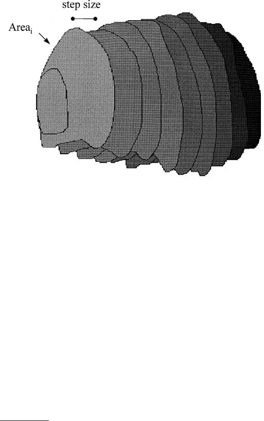
FIGURE 13.5 Outlines of cross-sectional images of the prostate used for planimetric volumetry of the prostate: transverse cross-sections obtained with a step size of 4 mm have been outlined by an expert observer, and the contribution of each section to the total volume is obtained by determining the area enclosed by the prostate contour. The volume is then determined by summarizing all contributions after multiplying them with the step size.

k=0

where a represents the position of the first section, n the number of sections, and h the step size, given by h = (b – a)/n, where b the position of the last section.

In general, three different forms of the approximation can be described, depending on the position of the section. The first form is known as the rectangular rule, and is presented in Equation 13.14. The midpoint rule is described by:

The trapezoidal rule is similar to the rectangular rule, except that it uses the average of the right-hand and left-hand Riemann sum:

The trapezoidal and midpoint rules are exact for a linear function and converge at least as fast as n–2, if the integrand has a continuous second derivative [14].

© 1999 by CRC Press LLC

FIGURE 13.6 An ellipsoid-shaped model of the prostate that was used for theoretical analysis of planimetric volumetry. Indicated are the intersection distance h and the scan angle α with the axis of the probe. (From R. G. Aarnink et al., Physiol. Meas., 16, 141-150, 1995. With permission.)

A number of parameters are associated with the accuracy of the approximation of the volume integral with a Riemann sum; first of all, the number of cross sections n is important as the sum converges with n–2: the more sections, the more accurate the results. Furthermore, the selection of the position of the first section is important. While the interval of integration is mostly well defined in theoretical analyses, for in vivo measurements, the first section is often less well defined. This means not only that the selection of this first section is random with the first possible section and this section increased with the step size, but also that sections can be missed. The last effect that may influence the numerical results is the effect of taking oblique sections, cross sections that are not taken perpendicular to the axis along which the intersection distance is measured. All the above assumes that every section Sk can be exactly determined.

The influence of the parameters associated with these kinds of measurements can be tested in a theoretical model. In a mathematical model with known exact volume or surface, the parameters — including step size, selection of the first section, and the scan angle — can be tested. Figure 13.6 shows a model used to model the prostate in two dimensions. It consists of a spheroid function with a length of the long axis of 50 mm and a length of the short axis of 40 mm. In mathematical form, this function can be described as:

with x0 half the diameter of the ellipse in x-direction (25 mm) and y0 half the diameter of the ellipse in y-direction (20 mm) and (xm, ym) the center point of the ellipse. The analytical solution of the integral to obtain the surface of this model is πx0 y0.

Figure 13.6 also reveals the possible influence of the parameters h and α. Figure 13.7 shows the results for varying the step size h between 4 mm and 16 mm corresponding to between 13 and 3 sections used for numerical integration as a function of the position of the first section. The first section is selected (at random) between the first coordinate of the function, and this coordinate plus the step size h. The sections were taken perpendicular to the long axis. From this study, which is fully described by Aarnink et al. [15], it was concluded that if the ratio of step size to the longest diameter is 6 or more, then the

© 1999 by CRC Press LLC