Supersymmetry. Theory, Experiment, and Cosmology

170 Phenomenology of supersymmetric models: supersymmetry at the quantum level

electroweak symmetry but they might lead also to undesirable charge or color breaking minima (we know that the quantum electrodynamics U (1) or the color SU (3) are good symmetries).

To simplify the discussion, we disregard the family structure and consider a single family (which could be any of the three; but since Yukawa couplings are larger for the third family, we choose it for illustration). The superpotential reads (cf. equations (5.1) and (5.2) of Chapter 5)

The tree-level potential V (0) = VF + VD + Vsof t must be complemented at least by the one-loop corrections. As we have seen in the preceding section, the complete one-loop potential reads, in the e ective potential approximation,

Avoiding instabilities in the flat directions of the scalar potential 171

where m2i is the field-dependent eigenvalue corresponding to a particle of spin si and Q is the renormalization scale8.

We will identify a F or D flat direction by specifying the supermultiplets which have a nonzero vev along the direction. In other words, along the direction (Φ1, Φ2, ..., Φn), the scalar components φ1, φ2, . . . , φn acquire a (possibly) nonvanishing vev.

Including the one-loop corrections is important in order to minimize the dependence on the renormalization scale Q : most of the dependence cancels between the running scalar masses which are present in the tree-level potential V (0) and the oneloop correction Ve(1) [173]. However, instead of using the full one-loop potential, we will use the following approximation scheme [71]: we take as a scale Q the largest field-dependent mass mˆ (φi) present in (7.52) in order to minimize the value of the one-loop correction. We then use the tree-level “improved” potential V (0) (mˆ (φi)).

We note that mˆ is in general the largest of the following two scales: a typical supersymmetric mass mSUSY (usually a squark mass) or a field-dependent mass in the form of a (gauge or Yukawa) coupling times the nonzero vev along the flat direction considered. For example, in the case of a direction which involves the field H20, we would have mˆ = λt H20 if we consider very large H20 vevs, and squark mass mSUSY otherwise (i.e. if H20 < mSUSY/λt).

Before discussing the potentially dangerous flat directions, let us review the case of the direction (H10, H20). This direction has already been considered in equation (5.15) of Chapter 5 for the discussion of electroweak symmetry breaking at tree level. The

as in equation (5.15) of Chapter 5 (m21 and m22 are defined as in (5.14) there and ϕ = Arg H20/H10 ). The condition for stability in this direction is the positivity condition:

Remember that this is evaluated at a scale Q of order λta (as long as Q is larger than mSUSY). If we start at the unification scale (or the scale of the underlying theory) MU , this constraint should be valid (otherwise the breaking occurs already in the underlying theory). When we go down in scale, we will eventually encounter the scale Qs where S becomes negative; we then have a Qs/hT .

Let us note that, if we were working solely with the tree level potential, the condition S < 0 would be the sign of a potential unbounded from below9. But this is obviously not the case here: for larger values of a (hence of the renormalization scale Q) the condition (7.54) is no longer satisfied. This is just a reflection of the fact that, had we worked with the complete one-loop potential (7.51), the large logs coming from (7.52) would prevent the field vev from going to infinitely large values.

8For obvious reasons we refrain from calling it µ in this Section

9This is why the type of direction that we study is often called an “unbounded from below direction” and denoted UFB [71]. We will refrain from doing so here.

High-energy vs. low-energy supersymmetry breaking 173

Finally, a word about cosmological arguments. It has been argued that, even in the cases where a charge or color breaking minimum deeper than the electroweak minimum appears, the time it takes to decay into this true vacuum ground state might be longer than the age of the Universe [77]. This indeed would make most of the problems discussed in this section innocuous and the corresponding bounds nonapplicable. One should, however, be guarded against cosmological arguments in the context of this discussion. In fact, as long as the cosmological constant problem is not solved, it is unadvisable to take at face value the expression of the potential in a (global or local) minimum. Whatever is the mechanism that is flushing (most of) the vacuum energy, it is di cult to imagine that it would distinguish between the electroweak symmetry breaking minimum and any other charge or color breaking minimum. Of course, this puts the whole issue of comparing ground states on somewhat shaky grounds. But, in the preceding analysis, we did not rely on any specific value of the vacuum energy whereas estimates of tunnelling e ects do. Other arguments that the system might choose the right minimum in the early Universe because of temperature corrections [265] would however be more reliable.

7.4High-energy vs. low-energy supersymmetry breaking

7.4.1Issues

As emphasized many times earlier, the issue of spontaneous supersymmetry breaking is central to this field: supersymmetry is not observed in the spectrum of fundamental particles. This means that, should supersymmetric particles be observed in high energy colliders, the focus of high energy physics would be to unravel the origin of supersymmetry breaking. We are not at this point yet but it is important to prepare the ground for such a task by studying general classes of supersymmetry breaking in order to understand their main experimental signatures, and how one can discriminate between them.

There are already quite a few constraints that a supersymmetry breaking scenario must obey. One may thus see how each scenario fares with respect to them. It is fair to say that not a single scenario passes all these tests magnum cum laude. We will return to this in more details in Chapter 12 and will only comment here on the possibly sensitive issues for each class of models.

7.4.2Gravity mediation. The example of gaugino condensation

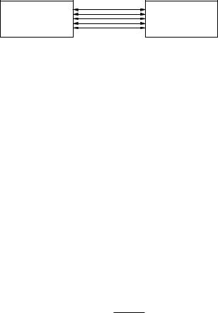
We have seen in Chapter 3 that it is phenomenologically undesirable to couple directly the source of supersymmetry-breaking to the quark and lepton fields. One is thus led to the general picture drawn in Fig. 7.6: an observable sector of quarks, leptons and their superpartners, a sector of supersymmetry breaking and an interaction that mediates between the two sectors.

In Chapter 6, the mediating interaction chosen was gravity. This has the advantage of really hiding the supersymmetry breaking sector: the coupling to the observable sector is the gravitational coupling κ−1 = m−P l2. A standard example is provided by the simple Polonyi model described in Section 6.3.2 of Chapter 6. In this model, the soft supersymmetry breaking terms are universal, i.e. they do not depend on the flavor. This is a welcome property because this satisfies more easily the constraints on flavor-changing neutral currents discussed in Section 6.7 of Chapter 6.

174 Phenomenology of supersymmetric models: supersymmetry at the quantum level

Fig. 7.6 General picture of supersymmetry breaking.

The rationale behind universality is the fact that gravity is flavor blind. In explicit theories that unify gravity with the standard gauge interactions, this is often not the case. We will return to this below. For the moment, we will describe a rather generic model of gravity mediation where supersymmetry is broken in the hidden sector by gaugino condensation.

Let us consider a theory where the gauge kinetic term fab is dynamical. To ensure universality (and gauge coupling unification), we assume that it is diagonal and expressed in terms of a single field S: fab = Sδab. In other words, the gauge kinetic terms read, from equation (6.25) of Chapter 6,

We will encounter such a field in the context of string models: it is the famous string dilaton. As in the string case, we assume that S does not appear in the superpotential. For the time being, we just note a few facts:

•The interaction terms (7.63) are of dimension 5. This means that there is a power

m−P 1 present which has been included in the definition of S (S is thus dimensionless). In other words, the S field has only gravitational couplings to the gauge fields, and to the other fields through radiative corrections.

•The gauge coupling is fixed by the vacuum expectation value of Re S:

Obviously, this only provides the value of the running gauge coupling at a given scale, typically the scale of the fundamental theory where the field S appears. Because of our assumptions, this corresponds also to the scale where the gauge couplings all have the same value, i.e. are unified, and we will denote this scale by MU .

•Since S does not appear in the superpotential, any minimum of the scalar potential is valid for any value of S: it corresponds to a flat direction of the potential. Hence the ground state value S remains undetermined: we may as well write it S, as long as some dynamics does not fix it.

We then assume that the theory considered involves a asymptotically free gauge interaction of group Gh under which the observable fields are neutral: the corresponding gauge fields Aµh and gauginos λh are part of the hidden sector.

As shown on Fig. 7.7, the associated gauge coupling explodes at a scale which is approximately given by

High-energy vs. low-energy supersymmetry breaking 175

g2(µ )

_

2/ S+S

Fig. 7.7 Evolution of the hidden sector gauge coupling with energy.

where b0 is the one-loop beta function coe cient associated with the hidden sector gauge symmetry considered and we have used (7.64). At this scale, the gauginos are strongly interacting and one expects that they will condense (we will develop in Chapter 8 more elaborate tools to study such dynamical e ects). On dimensional grounds, one expects the gaugino condensates of the hidden sector to be of order

It is clear that the replacement (7.66) in the supergravity Lagrangian induces some nontrivial potential for the S field: typically the four gaugino interaction present in the supergravity Lagrangian yields an exponentially decreasing potential for S. A safe way to infer the e ective theory below the condensation scale is to make use of the invariances of the complete theory [2, 353].

The symmetry that we use is K¨ahler invariance. We have seen in Chapter 6 that the

→ ¯ full supergravity Lagrangian is invariant under the K¨ahler transformation K F + F

if one performs a chiral U (1)K rotation (6.24) on the fermion fields. Choosing simply F = −2iα, this simply amounts to a R-symmetry11 where

This is, however, not a true invariance of the theory because it is anomalous. If we consider only the hidden sector, the divergence of the U (1)K current receives a contribution from the triangle anomaly associated with the gaugino fields:

11R-symmetries are global U (1) symmetries which do not commute with supersymmetry: supersymmetric partners transform di erently under R-symmetries. We have encountered them in Section 4.1 of Chapter 4 and will discuss them in more details in the next chapter, since they play, as we already see here, a central rˆole in the study of supersymmetry breaking. The transformation laws of the fields of a chiral supermultiplet are given in equation (C.43) of Appendix C (we take here r = 0).