1) Form a sparse distributed representation of the input

When you imagine an input to a region, think of it as a large number of bits. In a brain these would be axons from neurons. At any point in time some of these input

bits will be active (value 1) and others will be inactive (value 0). The percentage of

input bits that are active vary, say from 0% to 60%. The first thing an HTM region does is to convert this input into a new representation that is sparse. For example, the input might have 40% of its bits “on” but the new representation has just 2% of its bits “on”.

An HTM region is logically comprised of a set of columns. Each column is comprised of one or more cells. Columns may be logically arranged in a 2D array but this is not a requirement. Each column in a region is connected to a unique subset of the input bits (usually overlapping with other columns but never exactly the same subset of

input bits). As a result, different input patterns result in different levels of activation of the columns. The columns with the strongest activation inhibit, or deactivate, the columns with weaker activation. (The inhibition occurs within a radius that can

span from very local to the entire region.) The sparse representation of the input is encoded by which columns are active and which are inactive after inhibition. The

inhibition function is defined to achieve a relatively constant percentage of columns to be active, even when the number of input bits that are active varies significantly.

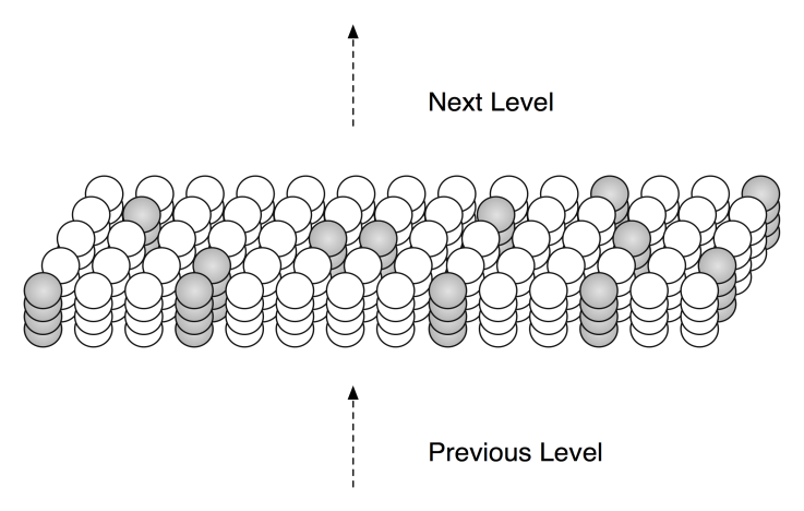
Figure 2.1: An HTM region consists of columns of cells. Only a small portion of a region is shown.

Each column of cells receives activation from a unique subset of the input. Columns with the strongest activation inhibit columns with weaker activation. The result is a sparse distributed representation of the input. The figure shows active columns in light grey. (When there is no prior state, every cell in the active columns will be active, as shown.)

Imagine now that the input pattern changes. If only a few input bits change, some columns will receive a few more or a few less inputs in the “on” state, but the set of active columns will not likely change much. Thus similar input patterns (ones that have a significant number of active bits in common) will map to a relatively stable set of active columns. How stable the encoding is depends greatly on what inputs

each column is connected to. These connections are learned via a method described later.

All these steps (learning the connections to each column from a subset of the inputs, determining the level of input to each column, and using inhibition to select a sparse set of active columns) is referred to as the “Spatial Pooler”. The term means

patterns that are “spatially” similar (meaning they share a large number of active bits) are “pooled” (meaning they are grouped together in a common representation).

2) Form a representation of the input in the context of previous inputs

The next function performed by a region is to convert the columnar representation of the input into a new representation that includes state, or context, from the past. The new representation is formed by activating a subset of the cells within each column, typically only one cell per column (Figure 2.2).

Consider hearing two spoken sentences, “I ate a pear” and “I have eight pears”. The words “ate” and “eight” are homonyms; they sound identical. We can be certain that at some point in the brain there are neurons that respond identically to the spoken words “ate” and “eight”. After all, identical sounds are entering the ear. However, we also can be certain that at another point in the brain the neurons that

respond to this input are different, in different contexts. The representations for the

sound “ate” will be different when you hear “I ate” vs. “I have eight”. Imagine that you have memorized the two sentences “I ate a pear” and “I have eight pears”.

Hearing “I ate…” leads to a different prediction than “I have eight…”. There must be

different internal representations after hearing “I ate” and “I have eight”.

This principle of encoding an input differently in different contexts is a universal feature of perception and action and is one of the most important functions of an HTM region. It is hard to overemphasize the importance of this capability.

Each column in an HTM region consists of multiple cells. All cells in a column get the same feed-forward input. Each cell in a column can be active or not active. By selecting different active cells in each active column, we can represent the exact

same input differently in different contexts. A specific example might help. Say every column has 4 cells and the representation of every input consists of 100 active columns. If only one cell per column is active at a time, we have 4^100 ways of representing the exact same input. The same input will always result in the same

100 columns being active, but in different contexts different cells in those columns will be active. Now we can represent the same input in a very large number of

contexts, but how unique will those different representations be? Nearly all

randomly chosen pairs of the 4^100 possible patterns will overlap by about 25 cells. Thus two representations of a particular input in different contexts will have about

25 cells in common and 75 cells that are different, making them easily distinguishable.

The general rule used by an HTM region is the following. When a column becomes active, it looks at all the cells in the column. If one or more cells in the column are already in the predictive state, only those cells become active. If no cells in the column are in the predictive state, then all the cells become active. You can think of it this way, if an input pattern is expected then the system confirms that expectation by activating only the cells in the predictive state. If the input pattern is unexpected then the system activates all cells in the column as if to say “the input occurred unexpectedly so all possible interpretations are valid”.

If there is no prior state, and therefore no context and prediction, all the cells in a column will become active when the column becomes active. This scenario is similar to hearing the first note in a song. Without context you usually can’t predict what will happen next; all options are available. If there is prior state but the input does not match what is expected, all the cells in the active column will become active. This determination is done on a column by column basis so a predictive match or mismatch is never an “all-or-nothing” event.

Figure 2.2: By activating a subset of cells in each column, an HTM region can represent the same input in many different contexts. Columns only activate predicted cells. Columns with no predicted cells activate all the cells in the column. The figure shows some columns with one cell active and some columns with all cells active.

.

As mentioned in the terminology section above, HTM cells can be in one of three states. If a cell is active due to feed-forward input we just use the term “active”. If the cell is active due to lateral connections to other nearby cells we say it is in the “predictive state” (Figure 2.3).