

EH_ch1_4
.pdfApplications |
65 |
that the mean a is unknown. In this case the natural statistical estimate of a is the sample mean,
t−1
at = t−1 pt−i .
i=0
Agents form the expectations accordingly, i.e., Et−1pt = Et−1pt+1 = at−1. Inserting these into the reduced form, we obtain
pt = α + (β0 + β1)at−1 + vt . |
(4.5) |
This is the law of motion for prices under the learning rule. Notice that if at converges to α/(1 − β0 − β1), then the price process converges to the stochastic steady state (4.4). We want to study whether this will in fact happen.
As was seen in the preceding example, the sample mean can be written in recursive form at = at−1 + t−1(pt − at−1). Inserting equation (4.5) into the recursive form, we obtain the dynamic equation
at = at−1 + t−1 α + (β0 + β1)at−1 − at−1 + vt . |
(4.6) |
This is a stochastic recursive algorithm that can be analyzed using stochastic approximation techniques. The basic technique was introduced in Chapter 2. The formal tools presented in Chapter 6 are applied to models of this type in Chapter 8.
We here outline the result that for this model, learning converges globally to the solution (4.4).3 Applying the stochastic approximation technique, we obtain the associated ODE
da = T (a) − a, dτ
where T (a) = α + (β0 + β1 − 1)a. It follows that at → α/(1 − β0 − β1), i.e., we have convergence to the stationary REE, provided β0 + β1 < 1, a condition which is satisfied by the model. Indeed, the global convergence theorem of Chapter 6 applies and there is convergence to this REE with probability 1.
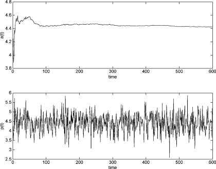
To illustrate these results, we provide an example simulation of equations (4.5)–(4.6). We set a2 = 1, b2 = −0.4, c1 = 1, and c2 = −.5. This leads
3The same techniques can be used to study whether the explosive solutions mentioned earlier can be attained as a result of a learning process. See Chapters 8 and 9.
66 |
View of the Landscape |
Figure 4.2.
to β0 = 0.6667 and β1 = 0.1111, and we also set α = 1. vt was assumed iid normal with standard deviation of 0.5. The initial value of at was set at a0 = 4. The top panel of Figure 4.2 illustrates convergence of the parameter estimate at to its RE value. The bottom panel shows the corresponding path for the market price pt . Of course, because of the intrinsic random shocks vt , the price path pt remains random in the limit, i.e., even after at has converged to
α/(1 − β0 − β1).
Numerous extensions to this analysis are of interest. First, the assumption of iid unobserved shocks is unnecessary. One could, for example, allow for observable shocks to any or all of the structural equations and the shocks could be allowed to follow specified exogenous processes. Agents would then use recursive least squares, as in Chapter 2, to estimate the dependence of pt on available information, and they would use their estimates to make appropriate forecasts. These issues are taken up in Chapter 8, where we show that there is convergence to the REE under slightly strengthened stability conditions.
As another extension, suppose that the previous assumption of a constant money supply m is replaced by a policy feedback rule in which money supply
Applications |
|
|
|
|
|
|
|
|
|
|
|
|
|
|
67 |
depends on the lagged price level |
|
|
|
|
|
|
|
|
|
||||||
|
|
|
|
mt = dI + dppt−1 + u4t . |
|
|
|
|
|
||||||
The reduced form now becomes |
|
|
|
|
|
|
|
|
|
||||||
|
= |
|
+ |
− |
|
+ |
t−1 |
|
+ |
t−1 |
|
+ |
+ |
|
(4.7) |
pt |
|
α |
|
δpt |
1 |
|
β0E |
pt |
|
β1E |
pt |
1 |
|
vt . |
|
There are now two rational expectations solutions of the form
pt = a + bpt−1 + vt ,
where b is a solution to the quadratic equation β1b2 + (β0 − 1)b + δ = 0.4 Provided |dp| is not too large, only one of the solutions will satisfy the stationarity condition |b| < 1.
Is this solution stable under learning? Again, it is now natural to assume that agents will recognize the dependence of price on lagged price in their “perceived law of motion.” In particular, suppose that agents have a perceived law of motion (PLM) of the same form as this REE, but do not know the RE values of a and b. Modeling the agents as econometricians, we can assume that they estimate the unknown parameters by least squares, regressing prices on lagged prices and an intercept, using the data that has been generated by the economy up to that point in time. Thus supposing that at time t − 1 their estimates are at−1, bt−1, they will make their forecasts of Et−1pt and Et−1pt+1 accordingly. Will their parameter estimates converge over time to the RE values? The results on the convergence of SRAs introduced in Chapter 2 can again be applied, even though the regressors are no longer exogenous, and the results are discussed in Chapters 8 and 9.
Finally, the inclusion of future expectations Et−1pt+1 in equation (4.3) leads to a crucial difference from the cobweb model of Chapter 2, namely that formally there are now multiple RE solutions. Although it can be shown that in the Sargent–Wallace “ad hoc” model of this section there is a unique stationary solution, there are other examples of the form (4.3) which have multiple stationary RE solutions. In such cases we will therefore want to examine systematically the stability under learning of the various solutions. This issue will be studied at length in Chapters 8 and 9.
4This is easily verified by computing Et−1pt = a + bpt−1 and Et−1pt+1 = a(1+ b) + b2 pt−1 and substituting into equation (4.7) and equating coefficients. We are assuming real solutions to the
quadratic.
68 |
View of the Landscape |
4.4 The Ramsey Model
The Ramsey growth model is widely used in macroeconomics. For simplicity we give a version which ignores population growth, technological progress, and depreciation.
An infinitely lived representative consumer maximizes intertemporal expected utility
∞
Et βt+i u(Ct+i )
i=0
subject to the budget constraints
Ct+i + Kt+1+i = wt+i + (1 + rt+i )Kt+i
for i = 0, . . . , ∞. Here Ct+i , Kt+i , wt+i , and rt+i denote consumption, capital, real wages, and interest rate in period t + i, respectively. 0 < β < 1 is the subjective discount factor. Labor supply is normalized at unity. We assume the household maximizes expected utility (rather than realized utility) because our households will not usually be assumed to have perfect foresight (also in later models random shocks will often be present).
The firm maximizes its profit
F (Kt+i , Nt+i ) − rt+i Kt+i − wt+i Nt+i
in each period. Here F (·, ·) is the production function with constant returns to scale and Nt+i denotes the labor input. Assuming perfect competition and market clearing, the first-order conditions for the firm yield the usual conditions that factors are paid their marginal products. These relations can be written
rt+i = f (Kt+i ),
wt+i = f (Kt+i ) − Kt+i f (Kt+i ),
where f (K/N) ≡ F (K/N, 1) and we have used the labor market clearing condition Nt+i = 1.5
5F (K, N ) = Nf (K/N ) because of constant returns to scale. Differentiating with respect to K yields ∂F /∂K = f (K/N ) and differentiating with respect to N yields ∂F /∂N = f (K/N ) − (K/N )f (K/N ). Note that constant returns to scale also implies that f (K/N ) is equal to output per worker.
Applications |
69 |
To maximize utility we substitute the household budget constraints into the objective function. By differentiation with respect to Kt , one obtains
u (Ct ) = βEt (1 + f (Kt+1))u (Ct+1) , Ct = Kt + f (Kt ) − Kt+1,
as the dynamical system. In the standard textbook analysis perfect foresight is assumed and we obtain a pair of nonlinear difference equations in Kt , Ct . For example, under the parametric assumptions F (K, N) = Kα N1−α and U (C) = C1−σ /(1 − σ ), we obtain
|
Kt 1 |
|
Kt Kα |
|
|
Ct . |
|
− |
|
|
|
|||
|
|
|
= |
|
β 1 |
+ |
|
|
Kα |
|
C )α−1 |
1/σ |
||
|
C |
+1 |
C |
α(K |
|
, |
||||||||
|
t |
t |
|
|
t + |
t |
|
|
t |
|
||||
|
|
+ |
= |
|
+ t |
− |
|
|
|
|
|
|
||
To illustrate the system we write it in the form |
|
|
||||||||||||
Ct+1 − Ct |
= Ctα β 1 + α(Kt + Ktα − Ct )α−1 |
1/σ − Ct , (4.8) |
||||||||||||
+ |
− |
Kt |
= |
t |
− |
|
, |
|
|
|
|
|
|
|
Kt 1 |
|
|
K |
Ct |
|
|
|
|
|
|
||||
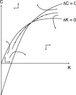
which is shown in Figure 4.3 and exhibits the familiar saddle point feature. It
is easily verified that there is a unique steady state |
¯ ¯ |
. The saddle point |
|
(K, C) |
|
properties of the steady state can be verified formally by computing the Jacobian
(K, C) |
and noting that the eigenvalues |
λ |
and λ satisfy |
of equation (4.8) at ¯ ¯ |
1 |
2 |
0 < λ1 < 1 < λ2. See, e.g., Azariadis (1993, pp. 72–75).
As seen in Figure 4.3, given K0, there is a unique choice of C0 such that
the path (K |
(K, C). |
Other paths explode, as illustrated in the |
t , Ct ) converges to |
¯ ¯ |
figure. These paths can be ruled out as perfect-foresight equilibria because they eventually violate nonnegativity or transversality conditions.
But suppose we drop the perfect-foresight assumption? The saddle path might then appear delicate, since agents would then be making forecasting errors. Formally, if agents form one-step-ahead expectations at each time t, we
have the system |
|
|
|
|
|
|
|
|
|
|
|
|
|
|
|
u (C ) |
|
βE |
(1 |
+ |
f |
(K |
|
))u |
(C |
t+1 |
) , |
(4.9) |
|||
t |
= |
|
t |
|
|
− |
t+1 |
|
|
|
|
|
|||
|
|
+ |
|
|
|
+ |
|
|
|
|
|
||||
Ct |
= |
Kt |
|
f (Kt ) |
|
Kt |
|
1 |
, |
|
|
|
|||
where Et (·) denotes the (in general nonrational) expectations of the households. This system defines a temporary equilibrium in which Ct and Kt+1 are determined, given these expectations and Kt . A reasonable learning rule will, of
70 |
View of the Landscape |
Figure 4.3.
course, respond to forecast errors and attempt to eliminate them, but it is not obvious whether such behavior will eventually lead the economy to the perfectforesight path or whether even small errors will drive the economy onto some unstable trajectory.
To analyze this question we will endow the agents with a forecast rule which determines Et (·) as a function of the observables. The forecast rule depends on parameters which will be updated each period on the basis of new observations. Such a system defines the economic dynamics under learning.
Perhaps surprisingly, it can be shown that the perfect-foresight saddle path for this economy is indeed locally learnable, i.e., is attained under a natural specification of the learning dynamics. We put off the demonstration of this result because of the relative complexity of this model, giving the formal details for the Ramsey model in the appendix at the end of this chapter. In Chapter 10 we show how to extend these results to the standard Real Business Cycle model, which is a well-known and widely used generalization of the Ramsey model incorporating variable labor supply and random productivity shocks.
More generally, realistic contemporary applied macroeconomic models are usually formulated as multivariate models in which the variables depend on their lags, on expectations of future variables, and on exogenous stochastic processes. In a neighborhood of a steady state these can be approximated by linear multivariate models, the solutions to which can be written as vector autoregressions. In Chapter 10 we show how to extend the techniques for studying least squares learning to multivariate frameworks and we apply the tools developed there to several models, including models with sunspot solutions as well as “regular” models like the Real Business Cycle model.
Applications |
71 |
4.5 The Diamond Growth Model
This model introduces physical capital goods into the overlapping generations structure. For an exposition of this model, known as the “Diamond model,” see, for example, Blanchard and Fischer (1989) or Romer (1995). To simplify the model we assume that the labor supply is held fixed and there is no monetary asset so that all saving is in the form of capital. Households supply (one unit of) labor when young and consume in both periods of their two-period lifetime. We also simplify by assuming that there is neither technical progress nor population growth.
Households born in period t maximize the utility function
|
C1−θ |
|
C1−θ |
||||||
Ut = |
|
1t |
|
+ β |
2,t+1 |
|
|||
1 |
− |
θ |
1 |
− |
θ |
||||
|
|
|
|
|
|
|
|||
subject to the budget constraint |
|
|
|
|
|
|
|
|
|
C2,t+1 = (1 + rt+1)(wt |
− C1t ), |
||||||||
where rt+1 is the interest rate in period t + 1 and wt is the real wage. Assuming perfect foresight, one can show that saving depends on the interest rate and is proportional to wt . Let s(rt+1) denote saving as a fraction of income wt (recall that there is a labor supply of 1). Note that s(r) is increasing or decreasing in r as θ is less than or greater than 1.
Since the old consume all of their income, the capital stock in period t + 1 is given by Kt+1 = s(rt+1)wt . Output is produced from capital and labor in the same way as in the Ramsey model, i.e., Yt = F (Kt , 1) ≡ f (Kt ). Under perfect competition, factors are paid their marginal products, so that rt = f (Kt ) and wt = f (Kt ) − Kt f (Kt ). We thus arrive at the key dynamic equation
Kt+1 = s(f (Kt+1)) f (Kt ) − Kt f (Kt ) .
The system starts at time t = 0 with an initial capital stock K0 owned by an initial old generation.
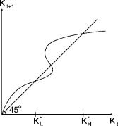
Under perfect foresight, there are various possible cases depending on the utility and production functions. For example, if the utility is logarithmic and the production function is Cobb–Douglas, there is a unique interior steady state to which the system converges from any initial capital stock K0 > 0. However, as is well known, for some choices of the utility and production functions, multiple interior steady states can exist, as illustrated in Figure 4.4. In fact, this figure shows a case where multiple Kt+1 can exist for a certain range of Kt . Under
72 |
View of the Landscape |
Figure 4.4.
perfect foresight, there would be no way to select between two alternative paths for an initial K0 in that range.
In contrast, consider the situation under learning. If households have an
expected interest rate re |
and save according to s(re |
), then the law of motion |
|
t+1 |
t+1 |
|
|
is instead |
|
|
|
Kt+1 = s(rte+1) f (Kt ) − Kt f (Kt ) . |
(4.10) |
||
To complete the model under learning we postulate a simple adaptive learning rule
rte+1 = rte + γt (rt − rte). |
(4.11) |
Substituting rt = f (Kt ), this leads to a two-dimensional dynamical system which will be analyzed in the appendix to this chapter. We state the result here: KL and KH are both stable under learning, though stability is only local and the eventual rest point will depend on the initial K0 and initial expectations r1e. The middle steady state is not stable.
4.6 A Model with Increasing Social Returns
A model with multiple steady states that are stable under adaptive learning can be developed using a simple extension of the OG production model introduced in Section 4.2. We develop this model at some length since it can also be used
Applications |
73 |
to illustrate the possibility of sunspot equilibria and the role of policy in models with multiple equilibria. This model will also be used to illustrate extensions and further phenomena in Parts IV and V.
4.6.1The Basic Framework
We return to the overlapping generations model discussed in Section 4.2. However, we replace the simple production function Qt = nt by the function
Qt = f (nt , Nt ),
where Nt denotes aggregate labor effort and represents a positive production externality. We assume f1 > 0, f2 > 0, and f11 < 0. Here Nt = nt , where is the total number of agents in the economy. is assumed large enough so that each agent has a negligible effect on Nt .
A specific formulation of f (nt , Nt ), given in Evans and Honkapohja (1995b) is as follows. The output Qt of an individual agent is assumed to depend on the individual’s labor input, which is partly mental, and on available complementary “ideas” for designs. There is a base level of standard design ideas I that always exist, but if aggregate output is sufficiently high, then the number of complementary ideas It , assumed generated in proportion to total labor effort and publicly available, exceeds I . If the dependence takes a Cobb– Douglas form, we have Qt = Anαt Itβ if It ≥ I and Qt = Anαt I β otherwise, with 0 < α < 1.
Suppose that agents have a unit endowment of time available to scan and absorb ideas, that the number of suitable ideas generated is λNt , and that it takes a units of time to receive and absorb a suitable idea. Then It = 1/(a + (λNt )−1) and we have
f (n, N) = Anα max I , λN/(1 + aλN) β .
Convenient features of this technology are that the externality is not present at low levels of N and that it is bounded as N → ∞.
Returning to the general formulation f (nt , Nt ), we can obtain the equilibrium equation as in the basic OG model. Agents are again assumed to maximize expected utility and the budget constraint is now that pt Qt = pt+1ct+1. Since each agent treats aggregate Nt as given, the first-order condition becomes
V |
(nt ) |
= |
E |
|
pt |
f1(nt , nt )U |
(ct 1). |
|
|||||||
|
|
|
t pt+1 |
|
+ |
||
In the basic overlapping generations model we analyzed expectations and learning in terms of the price of money. It is more convenient here to choose average
74 View of the Landscape
employment nt as the variable to be forecast. (Since nt is in 1–1 correspondence with the price level, this is an innocuous assumption.) We therefore reformulate
the model entirely in terms of nt . |
|
|
|
|
= M and pt /pt+1 = |
|
With a constant money supply M, we have pt Qt |
||||||
Qt+1/Qt . Using also ct+1 = Qt+1, we have |
|
|
|
|||
V (nt )f (nt , nt )/f1(nt , nt ) = Et f (nt+1, nt+1)U f (nt+1, nt+1) , |
||||||
or |
|
|
|
|
|
|
W |
(n ) |
= |
E G(n |
t+1 |
). |
(4.12) |
t |
t |
|
|
|||
It can be verified that W(nt ) is a strictly increasing function of nt . Solving for nt and assuming point expectations yields nt = F(net+1) for a suitable F. For our examples we will assume utility functions of the form
U (c) = c1−σ /(1 − σ ), V (n) = n1+ε/(1 + ε).
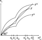
For appropriate σ and ε and parameter values for the production function above, one can obtain reduced form functions F which yield three interior steady states, as in the graph labeled F in Figure 4.5. Examples are given in Evans and Honkapohja (1995b) and below.
Employment levels nL < nU < nH correspond to low, medium, and high output levels. The steady states nL and nU can be interpreted as coordination failures since the steady states can be Pareto ranked and welfare is higher in nH than in either nL or nU . [For a proof see Evans and Honkapohja (1995b, Proposition 3).]
Figure 4.5.