

EH_ch1_4
.pdfIntroduction to the Techniques |
35 |
in our example, Xt follows an exogenous process, this is not at all essential. In particular, in the general framework, Xt can be permitted to follow a VAR (vector autoregression) with parameters that may depend on θt−1. This issue is discussed fully in Chapters 6 and 7.
The stochastic approximation approach associates an ordinary differential equation (ODE) with the SRA,
dθ = h(θ(τ )), dτ
where h(θ) is obtained as |
|
|
h(θ) = tlim |
EQ(t, θ, Xt ), |
(2.14) |
→∞ |
|
|
provided this limit exists. E denotes the expectation of Q(t, θ, Xt ), for θ fixed, taken over the invariant distribution of the stochastic process Xt . If Xt is not exogenous, but depends on θt−1, then one needs to use the more general formulation
|
h(θ) |
= t→∞ |
|
¯ t |
|
|
lim EQ t, θ, X (θ) , |
||||
where |
¯ t (θ) is the stochastic process for Xt |
obtained by holding θt−1 at the |
|||
|
X |
|
|
|
|
fixed value θt−1 = θ .
The stochastic approximation results show that the behavior of the SRA is well approximated by the behavior of the ODE for large t. In particular, possible limit points of the SRA correspond to locally stable equilibria of the ODE.
|
Before elaborating on this statement, it will be helpful to recall some basic |
||||||||||||||||||||||||||||||
stability results for ODEs. |
6 |
¯ is an equilibrium point of |
dθ/dτ |
= |
h(θ) |
if |
¯ |
= |
|||||||||||||||||||||||
¯ |
|
|
|
|
|
|
|
θ |
|
|
|
|
|
|
|
|
|
|
|
|
|
h(θ) |
|
||||||||
is said to be locally stable if for every |
ε > |
0, there exists |
δ > |
0 such that |
|||||||||||||||||||||||||||
0. θ |
|
|
¯ |
|
for all |
|
0 |
|
¯ |
|
|
|
|
|
|
|
|
|
|
|
|
|
|
|
|
|
|
||||
θ(τ ) |
|
< ε |
|
|
< δ |
. ¯ is said to be locally asymptotically stable |
|||||||||||||||||||||||||
|
|
|
θ |
|
θ( ) |
|
θ |
θ |
→ |
¯ for all |
|
0 |
|
in some neighborhood |
|||||||||||||||||
if ¯ is locally stable and in addition |
θ(τ ) |
θ( |
) |
||||||||||||||||||||||||||||
θ |
|
− |
|
|
|
|
|
|
− |
|
|
|
θ |
|
|
|
|
|
|
|
|
|
|
|
|
|
|||||
of θ |
|
|
|
|
θ is locally unstable if it is not locally stable. |
|
|
|
|
|
|
|
|||||||||||||||||||
¯ |
. We say that ¯ |
|
|
|
|
|
|
|
|
|
|
|
|
|
|
|
|
|
|
¯ |
is based on the |
||||||||||
|
It can be shown that the condition for local stability of |
||||||||||||||||||||||||||||||
derivative matrix (or “Jacobian”) |
|
|
¯ |
: |
|
|
|
|
|
|
|
|
θ |
|
|
|
|
|
|
||||||||||||
|
|
|
|
|
|
|
|
|
|
|
|
Dh(θ ) |
|
|
|
|
|
|
|
|
|
|
|
|
|
|
|
|
|
||
(i) |
If all eigenvalues of |
|
|
¯ |
|
have negative real parts, then |
|
¯ |
is a locally stable |
||||||||||||||||||||||
|
|
|
|
|
|
|
Dh(θ ) |
|
|
|
|
|
|
|
|
|
|
|
|
θ |
|
|
|
|
|
|
|
||||
equilibrium point of dθ/dτ = h(θ).
6Chapter 5 provides a review of stability results for ODEs.
36 |
|
|
View of the Landscape |
(ii) |
If some eigenvalue of |
Dh(θ ) has a positive real part, then θ is not a locally |
|
|
¯ |
¯ |
|
stable equilibrium point of dθ/dτ = h(θ).
We remark that in the cases not covered (where there are roots with zero real parts, but no root with a positive real part), more refined techniques are required to determine stability.
The stochastic approximation results can be stated as follows:
Under suitable assumptions, if |
¯ is a locally stable equilibrium point of the |
||||
ODE, then |
¯ |
|
θ |
¯ |
is not a |
is a possible point of convergence of the SRA. If |
|||||
|
θ |
|
|
θ |
|
locally stable equilibrium point of the ODE, then |
¯ is not a possible point of |
|
convergence of the SRA, i.e., θt → |
|
θ |
¯ with probability 0. |
||
|
θ |
|
Although the above statements appear fairly straightforward, the precise theorems are complex in detail. There are two reasons for this. First, there are vari-
ous ways to formalize the positive convergence result (when ¯ is a locally stable
θ
equilibrium point of the ODE). In certain cases, when there is a unique solution
and the ODE is globally stable, it can be shown that under the SRA, → ¯ with
θt θ probability 1 from any starting point. When there are multiple equilibria, however, such a strong result will not be possible, and indeed there may be multiple stable equilibria. In this case, if one artificially constrains θt to an appropri-
ate neighborhood of a locally stable equilibrium ¯ (using a so-called “projec-
θ
tion facility”), one can still obtain convergence with probability 1. Alternatively, without this device, one can, for example, show convergence with positive probability from appropriate starting points. The different ways of expressing local
stability of ¯ under the SRA are fully discussed in Chapter 6.
θ
Second, a careful statement is required of the technical assumptions under which the convergence conditions obtain. There are three broad classes of assumptions:
(i)regularity assumptions on Q,
(ii)conditions on the rate at which γt → 0,
(iii)assumptions on the properties of the stochastic process followed by the state variable Xt .
For condition (ii) on the gain sequence, a standard assumption is that γt = ∞ and γt2 < ∞. This is satisfied in particular by γt = t−1.
The precise statement of the conditions (i)–(iii) depends on the precise version of the stability or instability result, and in some cases, there are alternative sets of assumptions. Again, we will discuss these issues fully in Chapters 6 and 7. Finally, we remark that the formal instability result does not cover the
case in which |
¯ |
has roots with zero real parts but no postive roots. |
|
Dh(θ ) |
|
Introduction to the Techniques |
37 |
2.8 Application to the Cobweb Model
In this section we show how to apply the results of the previous section to the recursive formulation (2.11)–(2.12) of the cobweb model with learning to obtain the stability and instability results stated in Section 2.3. We begin by showing how equations (2.11)–(2.12) can be rewritten in the standard form (2.13) for the SRA. Then we explicitly compute the associated ODE using equation (2.14) and determine its stability conditions.
To show that the system can be put in standard form, we would like to define θt to include all the components of φt and Rt . However, there is a complication which arises in equation (2.11): on the right-hand side of the equation, the variable Rt rather than Rt−1 is present, while the standard form allows only the lagged value θt−1. To deal with this we define St−1 = Rt . The system (2.11)– (2.12) can then be rewritten
φt
St
1 |
|
1 |
|
|
|
= φt−1 + t−1 St−−1tzt−1 zt−1 |
(T (φt−1) − φt−1) + ηt |
||||
|
|
|
|
|
|
= St−1 + t− t |
+ |
|
|||
|
1 zt zt |
− St−1 . |
|||
,
(2.15)
(2.16)
Note that the second equation has been advanced by one period to accommodate the redating of Rt . This system is now implicitly in standard form with the following definitions of variables:
θt |
= vec 1φt |
St |
, |
||
|
= |
wt−1 |
|
|
|
Xt |
|
|
wt |
|
, |
|
|
|
ηt |
|
|
|
|
|
|
|
|
γt = t−1.
Recall that zt = ( 1 wt ). Thus all the components of zt and zt−1 have been included in Xt . Here vec denotes the matrix operator which stacks in order the columns of the matrix ( φt St ) into a column vector. The function Q(t, θt−1, Xt ) is now fully specified in equations (2.15)–(2.16). The first components of Q, giving the revisions to φt−1, are given by
Qφ (t, θt−1, Xt ) = S−1 zt−1 z −1(T (φt−1) − φt−1) + ηt ,
t−1 t

38 |
|
|
|
View of the Landscape |
and the remaining components are given by |
(zt zt |
− St−1) . |
||
QS (t, θt−1 |
, Xt ) = vec t + 1 |
|||
|
|
t |
|
|
Having shown that the system can be placed in standard SRA form, the next step is to compute the associated ODE. To do this we fix the value of θ in Q(t, θt−1, Xt ) and compute the expectation over Xt . Fixing the value of θ means fixing the values of φ and S, so that we have
hφ |
(φ, S) |
= t→∞ |
|
t |
− |
t−1 |
t |
−1 |
(T (φ) |
− |
φ) |
+ |
t |
|
|
|
lim |
ES |
1z |
|
z |
|
|
|
η |
, |
|||||
h |
(φ, S) |
lim |
|
|
|
E z |
t zt − |
S . |
|
|
|
|
|
||
|
|
|
|
|
|
|
|
||||||||
S |
= t→∞ t + 1 |
|
|
|
|
|
|
|
|||||||
h(θ) = vec(hφ (φ, S), hS (φ, S)), but it is easier to continue to work directly with the separate vector and matrix functions hφ (φ, S) and hS (φ, S). Since
Ezt zt |
= Ezt−1zt−1 = |
1 |
0 |
≡ M, |
0 |
||||
Ezt−1ηt = 0, and limt→∞ t/(t + 1) = 1, we obtain
hφ (φ, S) = S−1M(T (φ) − φ), hS (φ, S) = M − S.
We have therefore arrived at the associated ODE
dφ |
= S−1M(T (φ) − φ), |
(2.17) |
|
||
dτ |
||
dS |
= M − S. |
(2.18) |
|
||
dτ |
This system is recursive and the second set of equations is a globally stable system with S → M from any starting point. It follows that S−1M → I from any starting point, provided S is invertible along the path, and hence that the stability of the differential equations (2.17)–(2.18) is determined entirely by the stability of the smaller dimension system
dφ |
= T (φ) − φ. |
(2.19) |
dτ |
There are technical details required to establish this equivalence, since one must show that the possibility of a noninvertible S can be sidestepped. The technical arguments on this point are given in Chapter 6.
Introduction to the Techniques |
39 |
Recalling that φ = ( a b |
), note that equation (2.19) is identical to the dif- |
ferential equation (2.8) which defines E-stability. We have already seen that
¯ |
≡ |
¯ |
¯ |
is stable under equation (2.8) provided α < 1. Indeed, using the |
φ |
|
(a, b ) |
||
definition of T (φ) in equation (2.7), we can write
T (φ) − φ = |
µ |
+ (α − 1)I φ, |
δ |
where I is the identity matrix. Equation (2.19) is thus a linear differential equation with coefficient matrix (α − 1)I, all of whose eigenvalues are equal to
α − 1. |
¯ is thus a globally stable equilibrium point of equation (2.19) if |
α < |
1, |
|
φ |
|
but is unstable if α > 1. Applying the stochastic approximation results, it fol-
lows that under the SRA (2.15)–(2.16), (φt , St ) → |
¯ |
|
with probability 1 |
, |
|||||||
|
|
|
|
(φ, M) |
|
|
|
|
|
||
from any starting point, if α < 1. In particular, φ |
t → |
φ |
|
α < |
1. If |
α > |
1 |
, |
|||
|
|
|
|
¯ if |
|
|
|
||||
(φ, M) with probability 0. Since S |
t → |
M with probability 17 even if |
|||||||||
(φt , St ) → ¯ |
|
|
|
|
|
|
|
|
|
|
|
α > 1, it follows that φ |
φ |
|
|
|
|
|
|
|
|
|
|
t → ¯ with probability 0 if α > 1. Since the dynamic sys-
tem of least squares learning (2.1), (2.3), and (2.4) can be expressed as the SRA (2.15)–(2.16), we at last obtain the results stated in the theorem of Section 2.3.
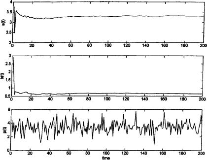
To illustrate results for the cobweb model, we exhibit a simulation with reduced form parameters µ = 5, δ = 1, and α = −0.5 (recall that in the cobweb model α < 0). The observable wt is a one-dimensional normal white noise process with standard deviation 1, and the unobservable white noise process ηt has standard deviation 0.5. We simulate equations (2.10), (2.11), and (2.12) with initial values a0 = 1, b0 = 2, and R0 equal to the 2 × 2 identity matrix. Figure 2.1 shows the trajectories for at , bt , and pt . Clearly, convergence to the REE values
¯ = |
10/3 and |
¯ |
= |
2 3 occurs quite rapidly. |
a |
|
|||
|
|
b |
|
/ |
2.9 The E-Stability Principle
In the remainder of the book we elaborate on the techniques described in this chapter and show how they can be extended to most standard theoretical and applied macroeconomic models. These models can have different types of equilibria such as ARMA or VAR processes, (noisy) k-cycles, or sunspots. It turns out that E-stability will play a central role in determining the stability of the REE under adaptive learning for the different models studied in this book.
7This is the strong law of large numbers applied to the process zt zt , and holds, in particular, if wt is an exogenous stationary VAR. Alternatively, it follows from applying the stochastic approximation techniques to the subsystem (2.16).
40 |
View of the Landscape |
Figure 2.1.
A general definition of E-stability is a straightforward extension of the example in this chapter. Starting with an economic model, we consider its REE solutions. Assume that any particular solution can be described as a stochastic
process with particular parameter values |
¯ |
Here |
φ |
might be, for example, the |
|
φ. |
|
|
parameters of an ARMA process or of a VAR or the mean values at the different points in a k-cycle. Under adaptive learning the agents are assumed not to
know |
¯ |
, but try to estimate it using data from the economy. This leads to statisti- |
|||
|
φ |
|
¯ as |
|
→ ∞ We |
cal estimates φt at time t, and the issue will be whether φt → |
t |
||||
|
|
|
φ |
. |
|
will in each case set up the problem as an SRA in order to examine the stability
of the solution ¯ . We will continue to find that stability of |
¯ under learning can |
|||||
φ |
|
|
|
|
|
φ |
be determined by the E-stability equation, i.e., by the stability of |
||||||
|
|
dφ |
= T (φ) − φ, |
(2.20) |
||
|
|
|
||||
|
|
dτ |
||||
in a neighborhood of ¯ |
where |
T (φ) |
is the mapping from the perceived law |
|||
φ, |
|
|
|
|
||
of motion φ to the implied actual law of motion T (φ). [Note that REEs corre-
Introduction to the Techniques |
|
41 |
spond to fixed points of T (φ).] Formally, |
¯ |
is said to be E-stable if it is locally |
|
φ |
|
asymptotically stable under the differential equation (2.20).
The correspondence between E-stability of an REE and its stability under adaptive learning we call the E-stability principle. In this book we primarily consider least squares and related statistical learning rules. Here there is strong support for the principle, and it also seems to hold for some non-statistical learning schemes. We regard the validity of the E-stability principle as an operating hypothesis.
It will become clear from the analysis of this book that the validity of the E-stability principle requires restricting attention to the standard case of gain decreasing to zero (in some cases a sufficiently small constant gain can be accommodated). Another assumption that is needed is that the information variables, on which the estimators are based, remain bounded. The general validity of the principle, i.e., general conditions under which the principle holds, remains to be determined.
An issue which will become increasingly important in our development is the precise specification of the learning rule followed by the agents. If we assume that our agents are behaving like econometricians, they will have to face some of the practical difficulties of econometricians, most importantly the issue of specifying the appropriate forecasting model. In our discussion of the cobweb model above, we implicitly assumed that the agents knew the correct asymptotic specification, i.e., they knew the appropriate vector of explanatory variables for forecasting next period’s price. We will continue to focus on this case in our analysis of more general economic models. However, it is reasonable to ask how misspecification would alter the results. Suppose agents overparameterize the solution, e.g., suppose the REE being examined follows an ARMA process and the agents fit a process with a higher AR or MA degree. Or suppose the REE being examined is a k-cycle and agents overfit with an nk-cycle. Will such overfitting alter the stability conditions? It turns out that this is an important issue to be examined particularly when there are multiple REEs. We can also consider the effect of agents underparameterizing an REEs solution. Here the agents cannot converge to the solution, but we can still ask if they converge and, if so, to what process?
The issue of overparameterization has a simple reflection in terms of E- stability. If agents overparameterize an REE solution, the solution can be rep-
resented as a higher-dimensional vector φ |
|
(φ1, φ2) with component values |
|||||||
¯ |
0 |
) |
at the REE in question. We can now look at the stability of |
|
|||||
(φ, |
|
|
|
|
˜ |
= |
|
|
|
|
|
|
|
d ˜ |
|
|
|
|
|
|
|
|
|
φ |
= |
˜ ˜ − |
˜ |
(2.21) |
|
|
|
|
|
|
|
T (φ) |
φ, |
||
dτ
42 |
|
View of the Landscape |
where |
˜ |
is the mapping from the perceived to the actual law of motion for this |
|
T |
|
expanded set of parameters. Indeed, it is useful to introduce some terminology
to represent this distinction. If the REE ¯ is locally stable under equation (2.20) |
||||||||
but |
¯ |
0 |
|
|
|
|
|
φ |
) |
is not locally stable under equation (2.21), then we say that it is weakly |
|||||||
|
(φ, |
|
|
¯ |
0 |
|
is also stable under equation (2.21), then we say that the |
|
E-stable, while if |
) |
|||||||
|
|
|
|
|
(φ, |
|
|
|
REE is strongly E-stable. As we will see, weak and strong E-stability govern whether the corresponding adaptive learning rules are stable. By expanding the dimension of φ appropriately, one can also allow for heterogeneous expectations across agents and determine whether allowing for heterogeneity alters the stability conditions for convergence of adaptive learning. In an analogous way, the concept of E-stability can also be adapted to determine conditions for the convergence of underparameterized learning rules by reducing the dimension of φ.
One could also consider structural heterogeneity, i.e., models in which individual agents respond differently to expectations. An open question is how E-stability can be adapted to such environments. Throughout the book we implicitly make the assumption of structural homogeneity, so that models such as equation (2.1) arise from a world in which the characteristics of individual agents are identical.
There is one more important conceptual issue that arises in connection with E-stability. In some papers, e.g., DeCanio (1979), Bray (1982), Evans (1983), and Evans (1985), iterations of the T -map are considered and the stability of an REE under these iterations is determined.8 Formally, this version of E-stability
replaces the differential equation (2.20) with the difference equation |
|
φN+1 = T (φN ), for N = 0, 1, 2, . . . . |
(2.22) |
In order to have a clear terminology, we will refer to the notion of stability determined by equation (2.22) as iterative E-stability, reserving the unmodified phrase “E-stability” for stability under the differential equation. Thus an REE
φ |
φ |
in a neighborhood of φ, we have φ |
φ |
¯ is iteratively E-stable if for all |
0 |
¯ |
N → ¯ |
under equation (2.22). |
|
|
|
Formally, there is a simple connection between E-stability and iterative E- |
|||
stability. The condition for |
¯ |
to be iteratively E-stable is that all eigenvalues of |
||
DT |
¯ |
|
φ |
|
lie inside the unit circle. In contrast, the E-stability condition, based on |
||||
|
(φ) |
|
|
|
8Iterations of the T -map were also considered in Lucas (1978). The term “expectational stability,” and the distinction between weak and strong (iterative) E-stability, were introduced in Evans (1983) and Evans (1985).
Introduction to the Techniques |
|
|
|
|
43 |
equation (2.20), is that all roots of DT |
¯ |
|
I |
have negative real parts; equiva- |
|
|
(φ) |
|
¯ |
must be less than 1. It follows |
|
lently, the real parts of all eigenvalues of DT |
|
||||
|
|
− |
(φ) |
|
|
immediately that iterative E-stability is a stricter condition than E-stability. For example, in the model (2.1) the E-stability condition, as we have shown, is that α < 1, while the iterative E-stability condition is |α| < 1.
We have seen that E-stability provides the condition for stability under adaptive learning rules such as least squares. What, therefore, do we learn from iterative E-stability? One rationale given in the papers cited was that it gave the condition for stability if agents kept fixed their perceived law of motion until a large amount of data was collected, revising their estimates infrequently rather than at each point in time. An alternative “eductive” rationale, also suggested in these papers, was that it described a process of learning taking place in “mental time,” as each agent considered the possible forecasts of other agents, iteratively eliminating those that correspond to dominated strategies. Using the game-theoretic notions of rationalizability and common knowledge, this approach was developed in Guesnerie (1992). It is discussed in Section 15.4 of Chapter 15. It has also been recently shown that iterative E-stability plays an important role for learning dynamics based on finite-memory rules in stochastic frameworks (see Honkapohja and Mitra, 1999).
Since this book focuses on adaptive learning, the appropriate stability conditions required are in almost all cases the E-stability conditions provided by the differential equation formulation.
2.10 Discussion of the Literature
In addition to the cobweb model, which we discussed throughout this chapter, the overlapping generations model and various linear models were the most frequently used frameworks in the early literature on learning.
Lucas (1986) is an early analysis of the stability of steady states under learning in an OG model. Grandmont (1985) considered the existence of deterministic cycles for the basic OG model. He also examined learning using the generalizations of adaptive expectations to nonlinear finite-memory forecast functions. Guesnerie and Woodford (1991) proposed a generalization to adaptive expectations by allowing possible convergence to deterministic cycles. Convergence of learning to sunspot equilibria in the basic OG model was first discovered by Woodford (1990).
Linear models more general than the cobweb model were considered under learning in the early literature. As already noted, Marcet and Sargent (1989c)
44 |
View of the Landscape |
proposed a general stochastic framework and the use of stochastic approximation techniques for the analysis of adaptive learning. Their paper includes several applications to well-known models. Margaritis (1987) applied Ljung’s method to the model of Bray (1982). Grandmont and Laroque (1991) examined learning in a deterministic linear model with a lagged endogenous variable for classes of finite-memory rules. Evans and Honkapohja (1994b) considered extensions of adaptive learning to stochastic linear models with multiple equilibria.
The more recent literature on adaptive learning will be referenced in the appropriate parts of this book. See also the surveys Evans and Honkapohja (1995a, 1999). The comments below provide references to approaches and literature that will not be covered in detail in later sections.
For Bayesian learning the first papers include Turnovsky (1969), Townsend (1978), Townsend (1983), and McLennan (1984). Bray and Kreps (1987) discussed rational learning and compared it to adaptive approaches. Nyarko (1991) showed in a monopoly model that Bayesian learning may fail to converge if the true parameters are outside the set of possible prior beliefs. Papers studying the implications of Bayesian learning include Feldman (1987b), Feldman (1987a), Vives (1993), Jun and Vives (1996), Bertocchi and Yong (1996), and Nyarko (1997). The collection Kurz (1997) contains central papers on a related notion of rational beliefs.
The study of finite-memory learning rules in nonstochastic models was initiated in Fuchs (1977), Fuchs (1979), Fuchs and Laroque (1976), and Tillmann (1983), and it was extended in Grandmont (1985) and Grandmont and Laroque (1986). These models can be viewed as a generalization of adaptive expectations. We remark that the finite-memory learning rules cannot converge to an REE in stochastic models, as noted by Evans and Honkapohja (1995c) and studied further by Honkapohja and Mitra (1999). Further references of expectations formation and learning in nonstochastic models are given in Section 7.2 of Chapter 7.
Learning in games has been subject to extensive work in recent years. Surveys are given in Marimon (1997) and Fudenberg and Levine (1998). Carton (1999) applied these techniques to the cobweb model. Kirman (1995) reviewed the closely related literature on learning in oligopoly models. Another related recent topic is social learning, see, e.g., Ellison and Fudenberg (1995) and Gale (1996).