

akgunduz
.pdf5.9. Appendix 5B |
105 |
5.9 Appendix 5B
Figure 5.9: # of classroom observations each month
Table 5.8: Wave 1 summary statistics of centers missing in wave 2
|
In Both Waves |
First Wave Only |
||
|
Daycare |
Playgroup |
Daycare |
Playgroup |
Emotional support |
5.011 |
5.054 |
5.048 |
4.874 |
|
(0.855) |
(0.865) |
(0.682) |
(0.919) |
Instructional support |
3.093 |
3.554 |
2.985 |
3.04 |
|
(1.072) |
(1.145) |
(0.904) |
(0.935) |
Average quality |
4.052 |
4.304 |
4.017 |
3.957 |
|
(0.863) |
(0.910) |
(0.657) |
(0.830) |
# of children |
9.726 |
10.073 |
8.585 |
9.549 |
|
(3.145) |
(3.982) |
(2.445) |
(3.460) |
# of adults |
1.968 |
2.214 |
1.858 |
2.071 |
|
(0.733) |
(0.858) |
(0.795) |
(0.857) |
Observations |
392 |
466 |
88 |
92 |
# of centers |
53 |
77 |
11 |
16 |
|
|
|
|
|
106 |
Chapter 5. |
Table 5.9: Summary statistics of center averages
|
Wave 1 |
Wave 2 |
||
|
Daycare |
Playgroup |
Daycare |
Playgroup |
Emotional support |
5.010 |
5.043 |
4.434 |
4.627 |
|
(0.659) |
(0.662) |
(0.469) |
(0.505) |
Instructional support |
3.117 |
3.543 |
2.594 |
3.248 |
|
(0.766) |
(0.855) |
(0.525) |
(0.580) |
Average quality |
4.064 |
4.293 |
3.514 |
3.937 |
|
(0.668) |
(0.713) |
(0.440) |
(0.488) |
Number of children |
9.644 |
10.149 |
9.122 |
10.464 |
|
(1.899) |
(2.804) |
(1.941) |
(2.443) |
Number of adults |
1.960 |
2.181 |
1.988 |
2.309 |
|
(0.532) |
(0.594) |
(0.599) |
(0.815) |
Number of centers |
53 |
77 |
53 |
77 |
|
|
|
|
|
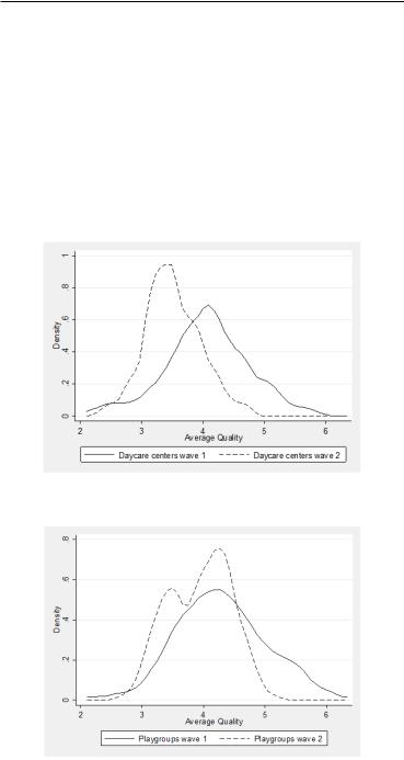
Figure 5.10: Distribution of child care quality in daycare centers’ (averages)
Figure 5.11: Distribution of child care quality in playgroups’ (averages)

5.9. Appendix 5B |
107 |
Table 5.10: Factor loadings for quality domains
|
Factor Loadings |
Emotional Support |
|
Positive climate |
0.7103 |
Teacher sensitivity |
0.7709 |
Regard for child perspectives |
0.3383 |
Behavior guidance |
0.6694 |
Instructional Support |
|
Facilitation of learning and development |
0.7664 |
Quality of feedback |
0.749 |
Language development |
0.7313 |
|
|
Table 5.11: Effects on individual quality indicators
|
Base |
Center Fixed Effects |
Structural indicators |
|
|
Number of children |
-1.0777*** |
-0.9734*** |
|
(0.3554) |
(0.3529) |
Number of adults |
-0.1143 |
-0.1247* |
|
(0.0855) |
(0.0754) |
Free play |
-0.0177 |
-0.0119 |
Emotional support indicators |
(0.0443) |
(0.0463) |
|
|
|
Positive climate |
-0.0740 |
-0.0549 |
|
(0.1097) |
(0.0984) |
Teacher sensitivity |
-0.1767* |
-0.1244 |
|
(0.1026) |
(0.0989) |
Regard for child perspectives |
-0.2184* |
-0.2569** |
|
(0.1270) |
(0.1243) |
Behavior guidance |
-0.2550** |
-0.2609** |
Instructional support indicators |
(0.1070) |
(0.1025) |
|
|
|
Facilitation of learning and development |
-0.4066*** |
-0.4509*** |
|
(0.1209) |
(0.1164) |
Quality of feedback |
-0.2115* |
-0.2348** |
|
(0.1078) |
(0.0986) |
Language development |
-0.0041 |
-0.0660 |
Factor variables |
(0.1137) |
(0.1020) |
|
|
|
Emotional support |
-0.1656** |
-0.1445* |
|
(0.0832) |
(0.0758) |
Instructional support |
-0.1779** |
-0.2136*** |
|
(0.0811) |
(0.0733) |
Robust standard errors are used in both regressions.
*** p<0.01, ** p<0.05, * p<0.1

108 |
|
|
|
|
|
Chapter 5. |
Table 5.12: QREG, CIC and TDID estimates using center averages |
||||||
|
|
|
|
|
|
|
|
|
|
|
Quantile |
|
|
|
|
|
|
|
|
|
QREG |
Avg. effect |
0.1 |
0.25 |
0.5 |
0.75 |
0.9 |
|
|
|
|
|
|
|
Effect size |
|
-0.0608 |
-0.0521 |
-0.3125 |
-0.5885*** |
-0.1644 |
S.E. |
|
(0.3552) |
(0.1597) |
(0.2108) |
(0.1770) |
(0.2010) |
TDID | FE |
|
|
|
|
|
|
Effect size |
-0.2441* |
-0.0170 |
-0.4219** |
-0.6501*** |
-0.239 |
-0.0806 |
S.E. |
(0.1332) |
(0.1525) |
(0.1881) |
(0.2070) |
(0.1757) |
(0.2942) |
CIC |
|
|
|
|
|
|
Effect size |
-0.3215** |
-0.0833 |
-0.3750 |
-0.6250** |
-0.5000** |
-0.2500 |
S.E. Bootstrap |
(0.1759) |
(0.3933) |
(0.3401) |
(0.3082) |
(0.1913) |
(0.2338) |
Standard errors in parenthesis. 200 repetitions are used for the bootstrapped standard error errors. ***p<0.01, ** p<0.05, * p<0.1. The QREG model includes 14 year-month fixed effects. The TDID model includes 129 centers fixed-effects and 14 year-month fixed effects. The date of the first class observation in each wave is used to construct year-month fixed-effects.
Chapter 6
Child Care Quality and the Labor
Supply of Married Women
6.1 Introduction
Increasing female employment has been a major policy goal for some time. The main instrument in stimulating female labor supply has been child care subsidies designed to increase access and affordability of child care for mothers of young children. Recent elasticity estimates form the Netherlands, Sweden and Norway show insignificant or small effects from further decreases in child care prices (Wetzels, 2005; Lundin et al., 2008; Kornstad and Thoresen, 2007). Literature is silent on how child care quality, which has become a policy goal in itself, affects female labor supply.
Especially in Western Europe, high labor force participation rates combined with low child care prices have begun to limit the effectiveness of further subsidies to raise labor supply. Recent elasticity estimates from the Netherlands, Sweden and Norway show insignificant or small effects from further decreases in child care prices (Wetzels, 2005; Lundin et al., 2008; Kornstad and Thoresen, 2007). Limited increases from lower child care prices do not imply, however, that female labor supply has reached a ceiling or has equalled that of men. Female participation figures are closer to men’s in Western Europe, but women work fewer hours. Apparently, even with very low prices mothers are unwilling to use child care and increase working hours further, which may be related to concerns over the quality of care children receive.
In this chapter, we estimate the effect of child care quality on the labor supply of
109
110 |
Chapter 6. |
married women. The focus is on the Netherlands where part-time work is common among women (Freeman, 1998), we study the choice between non-participation, parttime employment and full-time employment.
To analyze the role of child care quality in labor supply, we utilize a mixed multinomial logit model that accounts for unobserved heterogeneity. The primary dataset is Pre-Cool, a panel survey for the period 2010-2012 on child care quality in the Netherlands that also includes information on parents’ background characteristics and employment. The estimation relies on the surprisingly large variation across child care centers’ quality, which is mostly explained by the location of the market that they are placed in. The Pre-Cool data is supplemented with administrative data from 2009 wave of the Labor Market Panel of Dutch Statistics which is used to predict the wages of the Pre-Cool sample.
Our main findings are the following. First, we find no link between child care quality and married women’s labor supply. In line with the previous literature, center prices have a negative effect on labor supply. We also find a fairly large wage elasticity for Dutch women with young children.
The mixed logit model has previously been used to estimate the effect of child care prices on labor supply. The present chapter adds child care quality to the existing structural labor supply models (Powell, 2002; Tekin, 2007; Kornstad and Thoresen, 2007). While the importance of quality is raised in relation to its effect on child development in empirical work, the link between labor supply and quality is only noted in theory without an empirical application (Blau and Currie, 2006). Quality is typically treated as a latent and constant variable, since observations of child care quality is scarce (Ribar, 1995). Despite the theoretically proposed positive link between child care quality and female labor supply, our results seem to suggest that parents are unable to take child care quality into account in their employment and child care choices.
In the next section, we describe the mixed logit model we use to analyze the impact of child care quality and prices on female labor supply. The third section introduces the two datasets used to estimate the model. Section 4 provides the estimation results and simulated elasticities. Section 5 concludes.
6.2. Theory and Methodology |
111 |
6.2 Theory and Methodology
We use a discrete choice model to analyze mothers’ decisions with regard to employment and child care type. For tractability, we assume the mother’s decision to work occurs after her partner’s income is known (Killingsworth and Heckman, 1986). Having a higher income partner is thus one of the variables in a vector of observable personal characteristics X. Given X and u1, a mother’s utility within category k is a function of her leisure time L, the quality of her child Q, consumption C and unpaid hours of child care Hpu . The category k is defined by the categorical, discrete variable
K = 1...k, where each category denotes a different employment status. Categories may have other unobserved characteristics which can influence utility. For example, choosing a state with full-time work might be stigmatizing for some women regardless of the quality of child care. The unobservable characteristics are given by u1. The resulting utility function is given by:
U = U(L,Q,C,K;X,u1) |
(6.1) |
The budget constraint of the household depends on the wage w which varies between full-time wf and part-time employment wp, the price of child care that is pc per hour of center care Hpc and pi per hour of informal care Hpi and other income N. Each woman can fall within one of the five categories given in Table 6.1. We only distinguish between employed women for child care use, even though there are some women who also use formal child care despite having reported non-participation.
The budget constraint for the maximization problem depends on the category chosen. Each constraint depends on the wage w which varies between full-time wf and part-time employment wp, price of child care that is pc per hour of center care
Hpc and pi per hour of informal care Hpi and income from sources other than wages
N. We constructed the five alternative categories presented in table 6.1, each for a different level of employment and child care type.
Child quality is a function of the hours of paid and unpaid child care, the hours the mother spends with the child during her leisure L, and the paid child care quality
A. A contentious issue is how to include child care quality. Previous studies have treated child care quality as a variable maximized by the mother in the utility function, allowing for its treatment as a latent variable that does not appear in the indirect utility function. We do not assume that child care quality is maximized by the mother the
112 |
Chapter 6. |
way employment and leisure hours are. Instead, mothers are assumed to use the child care with a given quality A that is available to them. This does not mean that two mothers living in the same area will have the exact quality child care. Some parents will be able to choose better quality child care because they can distinguish between high and low quality child care. However, the preference for high quality over low quality is universal for all parents the same way higher wages are always preferred over lower wages. We take into account personal characteristics X such as education that might affect the ability of the parents to distinguish between high and low quality child care when we estimate the quality values.
Q = Q(Hpi ,Hpf ,L;X,A) |
(6.2) |
A time constraint is needed to close the model. Since we do not utilize time-use data, we cannot distinguish between time that the mother actually spends with the child and her leisure. Following the previous literature, the basic time constraint is given by equation (6.3) where the hours work E equals the hours of unpaid and paid child care (Ribar, 1995; Tekin, 2007).
L = 1 E = 1 (Hpf + Hpi ) |
(6.3) |
The outcome of interest in the empirical model is not utility itself, which is unobserved. Instead, we are interested in estimating the probability of choosing category k. Assuming that the mother maximizes her utility subject to (6.3), she chooses a specific value for L, Hpi , Hpf and C in each category. To estimate the model, we specify a linear approximation for the indirect utility function in category k for individual i given by:
Table 6.1: Category Definitions and Budget Constraints
|
Employment |
Center Child care |
Budget Constraint |
1 |
No |
No |
C = N |
2 |
Part-time |
No |
C = N + wp piHpi |
3 |
Part-time |
Yes |
C = N + wp pf Hpc |
4 |
Full-time |
No |
C = N + wf piHpi |
5 |
Full-time |
Yes |
C = N + wf pf Hpc |
6.2. Theory and Methodology |
113 |
Vik = Xib + a1 pik + a2wik + a3Aik + eik |
(6.4) |
Equation (6.4) defines the indirect utility function that can be estimated given
Xi, pik, wik and Aik. Adding an unobserved random component eik results in an additive random-utility model that can be estimated using a multinomial logit model (Cameron and Trivedi, 2009). The category k is observed if k has the highest utility of the alternatives. In line with Blau and Hagy (1998), equation (6.5) states the model formally by defining the probability that outcome k is observed as the probability that category k results in a higher level of utility than all other alternatives.
Pr(k) = Pr(Uk > Uj) = Pr(ek ej > a1(pj pk) + a2(wj wk) + a3(Aj Ak)
(6.5) So far, we have not made any assumptions about the structure of the error term eik. The basic multinomial logit model assumes independence of irrelevant alterna-
tives and that the error term is independently and identically distributed extreme value type 1. In line with the mixed logit model introduced in Revelt and Train (1998) we can add random components to the coefficients to capture heterogeneity in tastes. While we could allow all coefficients to vary randomly, this is generally not feasible in applied work due to computational constraints. Previous labor supply models using a similar random coefficient specification generally allow for the coefficient on income or leisure to have a random component (Van Soest, 1995; Haan, 2006). We allow for two variables’ coefficients to have random components: quality and wages. Quality, wage and price variables are in the vector a of the variables that are alternative specific. The coefficients of quality and wage variables then take the form ai = a + Ji where ai has a multivariate normal distribution with mean a, which allows the estimation of the distribution and covariance matrix of ai. Since parents who are particularly concerned with quality may have more or less taste for income, the random components are allowed to be correlated. The alternative invariant individual characteristics X have fixed coefficients. The resulting mixed logit estimation for the probability of observing choice k given observed characteristics Xit and alternative specific characteristics Sitk can be written as:

114 |
|
Chapter 6. |
P(kjXit ,ait ) = |
exp(Xit bk + aiSitk) |
(6.6) |
k |
||
|
å exp(Xit bj + aiSit j) |
|
|
j=1 |
|
In order to identify the model, the base category (non-participation) coefficients are all set to 0. To capture category effects, we introduce a fixed effect for each category. We expect that there are fixed costs associated with each category, whether it is unpaid care or travel to work and category specific fixed effects are meant to capture those.
The difficulty in estimating the model lies in assigning values to the random components. The likelihood function for individual i observed in category k shown by equation (6.6) can be expressed as an integral over the entire distribution of the unobserved heterogeneity terms as shown in equation (6.7). To estimate the likelihood function, recent literature has generally followed Train (2009) in using simulated maximum likelihood based on Halton sequences. The premise of the simulated maximum likelihood estimation is to make a large number of quasi-random draws of Ji to determine the distribution that maximizes the likelihood function given in equation (6.7). 1
|
N |
¥ T k |
exp(Xit bk + aiSitk) |
|
|
|
P(k Xitk,ai) = Õ |
ÕÕ |
f (ai)d(ai) |
(6.7) |
|||
|
||||||
j |
i=1 Z ¥ t=1 j=1 |
k |
|
|
||
|
|
|
å exp(Xit bj + aiSit j) |
|
|
|
j=1
In order to estimate (6.6), we need values for wage, child care price and quality. These three variables are estimated using a reduced-form approximation of the demand functions. For identification of wages, quality and prices, we use the province that the parents are residing in as the exclusion restrictions (Tekin, 2007). Previous labor supply models have also used education variables to identify effects, but education is likely to have a positive effect on taste for employment which would imply that the elasticities for income become inflated when they are omitted from the main model (Keane, 2011). The underlying assumption for using province as the exclusion restriction is that the region that parents reside in does not affect the indirect utility function except through the available quality, price and wage levels. Labor markets and child care markets where wages, prices and quality are determined are expected to be geographically constrained, leading to significant variation
1the model is estimated using the STATA code made available by Hole (2007).