akgunduz

municipality fixed effects in order to control for market heterogeneity, which further increases the treatment effect to -0.22. In the fourth model, municipality interactions with the center type are added to control for market heterogeneity differences between daycare centers and playgroups. The results show little difference compared to model (3). The final model adds center fixed effects and shows a similar treatment effect to models with municipality controls.

We report robust standard errors and standard errors clustered at different higher levels of aggregation. Specifically, we use standard errors clustered at the centerwave, center and municipality level. Bertrand et al. (2004) note that serial correlation in time series data can cause overrejection in DD estimates, but our data is only comprised of two waves. While the effects sizes do not vary between the models with and without center and municipality fixed effects by much, clustering seems to increase the size of the standard errors as expected. Model 5 likely provides the most reliable estimate since it takes into account center heterogeneity and includes yearmonth fixed effects. In that case, the coefficient is highly significant when robust standard errors or clustering is used per center in each wave. However, standard errors rise when they are clustered at the center or municipality level.

Table 5.3: Effects of the 2012 subsidy reduction on average quality

Standard errors in parenthesis *** p<0.01, ** p<0.05, * p<0.1 There are 260 clusters at the time x center, 130 clusters at the center and 38 clusters at the municipality levels.

The results in Table 5.3 show a generally negative effect from the subsidy reduction on daycare centers’ quality. When DD models are fitted for all seven dimensions and instructional and emotional domains’ factor scores separately, the coefficients are negative for both domains, and all individual dimensions as shown in table 5.11

in Appendix 5B. The effect sizes are larger and more significant for the instructional support domain. The larger effect on instructional support seems to be driven by facilitation of learning and development dimension. Previous literature has shown that instructional support measures are particularly important for school readiness (Mashburn et al., 2008). Especially in the Netherlands, quality scores were already below average for instructional support. Further decreases are more likely to have negative consequences on long term outcomes.

The effect on mean quality of 0.2 is around a third of the standard deviation of average quality. For the US, Duncan (2003) finds that a reduction of one standard deviation in process quality is associated with a decrease of a tenth of a standard deviation of cognitive scores for small children. If the association between child care quality and child development in the US is similar to the Netherlands, the subsidy reduction would have decreased cognitive development of Dutch children attending daycares by 3% of a standard deviation. The negative effects we find might be transitory since we are only looking at the year immediately after the subsidy reduction. In the case of child care however, short or long-term effects may be equally significant. Low quality care for even a few years may have long lasting effects on children currently in child care, since the formal child care period is only until the age of 4 in the Netherlands.

While the results suggest that process quality declined as a result of the subsidy cuts, there also appear to be effects on more structural factors such as the number of children and adults in each classroom. Table 5.11 in Appendix 5B shows that the number of children and adults in each classroom declined. This might be a result of the decline in demand for which the centers have not yet adjusted the number of groups. Since group size has a negative impact on process quality, including these variables in the main regression slightly increases the coefficient which remains below 0.25. Finally, we checked whether the activity assessed by the Pre-Cool observer varied significantly by using the most common activity, free play, as a dependent variable. In that case, there do not appear to be any significant effects.

As an informal check on whether there was significant sample selection, Table 5.8 in Appendix 5B separately shows the wave 1 quality values of centers that are not in wave 2. There is no evidence of sample selection for daycare centers where the average wave 1 quality is almost the same as the observed sample. Among playgroups, centers that are not in wave 2 have lower average quality. Simply including these centers in the regressions results in slightly larger treatment effects.

5.6 Estimating quantile effects

5.6.1Empirical methodology

Next, we estimate models that takes into account the shift in the full distribution of quality values. First, we implement the changes-in-changes (CIC) model of Athey and Imbens (2006) and then confirm the results using the recentered influence function method of Firpo et al. (2009). The non-linear models relax the additivity assumption in the DD model and compare the changes in distributions rather than the means. To compare the results, we also fitted the quantile difference-in-differences (QDID) model. The quantile models have two potential advantages over the linear DD model in our case. First is the shift in the distributions of both playgroups and daycare centers’ quality values from wave 1 to wave 2. Second, daycare centers with different starting levels of quality in wave 1 might react differently to the subsidy cut.

The CIC model, changes in the variance of outcomes over time within treatment and control groups are explained through changes in the production function for the outcome defined by Y = hI (u,t) where u are unobserved characteristics at time t. The restriction of the function h(.) is that it is monotonic and increasing in u. In contrast to the DD model which ignores changes in the distribution of outcomes and provides identification through the change in conditional means, identification in the CIC model is based on the full distribution of control and treatment groups before and after the treatment. Given an outcome value in the treatment group in the first wave

Y10 and its associated quantile q, we first find the matching value in the first wave control group Y00 = Y10 with its associated quantile q0. Taking into account the change in the cumulative distribution function of the control group in the second wave, we can find the second wave value Y01 at quantile q0. The difference between the first and second wave values of the control group at quantile q0 ,s used by the counterfactual change for quantile q of the treatment group. Athey and Imbens (2006) show that the complete counterfactual distribution of the treatment group FY N can be obtained using equation 5.3. Once the complete counterfactual distribution is constructed, the average treatment effect can be calculated by taking the difference between the realized distribution of the treatment group and the counterfactual distribution.

Finally, we apply the recentered influence function method of Firpo et al. (2009),

we follow the application of Havnes and Mogstad (2011b) of the threshold DD (TDID) model. Firpo et al. (2009)’s shows that the unconditional quantile regression can be redefined as a linear regression where the dependent variable is the probability that an observed outcome is greater than a given level. By estimating equation 5.4 using OLS, we can then determine the effect of the subsidy reduction Ii on the possibility thatthe observed quality Yit is greater than the quality level at y.

5.6.2Results

Using the CIC and threshold DD methods, the full counterfactual distribution has to be estimated and it is possible to calculate the effects at different quantiles. Since the standard errors cannot be clustered in CIC and threshold DD models, the standard errors for these models will be underestimated. The analytical standard errors that Athey and Imbens (2006) provide do not differ significantly from bootstrapped standard errors. Similarly, the robust standard errors used for the TDID model are similar in size to the bootstrapped standard errors. Due to the finite sample size, bootstrapped and analytical standard errors are about identical.

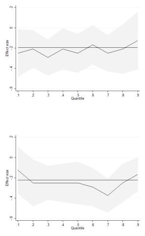
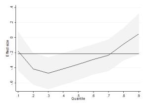
Table 5.5 shows the average treatment effect along with the estimated effects at 10th, 25th, 50th, 75th and 90th quantiles. We also plot the quantile effects using 0.1 intervals. The average treatment effect is similar in size to the estimates from the linear DD models in both the CIC and TDID models. The coefficients for the different quantiles show that the effects are larger in the middle of the quality distribution, especially in the TDID and QDID models. The linear quantile (QDID) model suggests that the effects are strong also at the bottom of the quality distribution, but given the large change in distributions from wave 1 to wave 2, the results from the non-linear models may be more informative.

A possible explanation for the heterogenous effects may be that the low quality child care centers simply do not have any more room to cut costs and lower quality given the current regulations. At the same time, highest quality centers may also be catering to parents with strong tastes for child care quality or very high income and thus low demand elasticity. A more straightforward explanation is that the subsidy cuts were not homogenous for all income groups. If higher income parents also use higher quality care, the heterogeneous effects would reflect the larger cuts for middle

Figure 5.6: Quantile Effects - QDID

Figure 5.7: Quantile Effects - CIC

and higher income families.

We cannot use clustered standard errors for quantile effects. To allow for common effects at the center level, we average classroom quality per center and fit the CIC and threshold DD models at the center level instead of the classroom level. The results are presented in table 5.12 in Appendix 5B. The average treatment effects are larger when center averages are used but the significance levels are at the 5% and 10% levels rather than 1% due to the larger standard errors. The quantile effects remain

Figure 5.8: Quantile Effects - TDID

significant at the 0.25 and 0.5 quantiles but turn insignificant at the 0.75 quantile for the threshold DD model using center averages..

5.7 Conclusions

We examine the impact of child care cut reduction on child care quality in the Netherlands using a natural experiment with playgroups as the control group. The results show that process quality in Dutch daycare centers declined as a result of the subsidy cut. The baseline treatment effects estimated using linear DD models are robust across linear DD models, synthetic controls, threshold DD and CIC models. Estimates by quantiles of quality show that the effects are concentrated in the middle of the quality distribution.

Currently there appear to be two policy objectives pulling in opposite directions when it comes to child care subsidies and child care services in general. On the one hand, research showing significant positive gains in future outcomes of children attending high quality care has led to discussions on extending the coverage of child care services. On the other hand, austerity measures in many European countries is leading to cuts in child care spending. These cuts are assumed to have low costs since the labor supply effects are generally found to be limited. However, cost on child care quality from cuts are typically ignored, since there is a lack of empirical evidence in this area.

An interesting question to consider is how increases in subsidies would influence child care quality. A straightforward interpretation of the Dutch experience would be that an increase in subsidies would raise both quality and coverage. However, there is no evidence to suggest that the effects of child care subsidies are symmetric. Higher demand as a result of child care subsidies can lead to higher prices if supply does not adjust accordingly and parents’ choices are limited. The effects of subsidy increases would need to be considered within the specific market in which they are implemented. Easy entry into the market to allow for more parental choice and regulations on prices may be required to realize concurrent increases in child care centers’ coverage and quality. Alternatively, more direct options to increase quality such as structural regulations or changes in the pedagogic curriculum can be explored.

5.8 Appendix 5A

In this Appendix, we calculate the net income and net child care costs of var-

ious household types to see what the net increase in monthly child care costs are.

To calculate net family incomes, the MICROTAX programme of the Dutch Central

Planning Bureau (CPB) is used. We assume in all cases that the total monthly hours

of child care used is 120. In table 1, net costs are calculated for a single parent family,

a couple with one parent working full time and the other part-time and a dual income

family. In table 2, same calculations are presented for families with two childen in

formal child care.

Table 5.6: Child care costs of median income households with one child

Table 5.7: Child care costs of median income households with two children