Higher Mathematics. Part 3

8.2. Evaluate the surface integrals of the second type

I = ∫∫ Pdydz + Qdxdz + Rdxdy, where σ is the upper side of a plane part α

σ

(triangle) which is placed between coordinate planes (Table 8.2).

202

Micromodule 9

BASIC THEORETICAL INFORMATION.

ELEMENTS OF FIELD THEORY

Scalar and vector fields. Gradient of a scalar field. Directional derivative. Flux, circulation, divergence, rotation of the vector field. Gauss — Ostrogradsky formula. Stokes’ formula. Hamiltonian operator. Potential, solenoidal, harmonic fields. Differential operations of the first and second orders.

Key words: Scalar and vector field — скалярне і векторне поле, gradient — градієнт, directional derivative — похідна за напрямом, flux — потік, circulation — циркуляція, divergence — дивергенція, rotation — ротор, Hamiltonian operator — оператор Гамільтона, potential — потенціал, solenoidal —

соленоідальний, harmonic — гармонічний.

Literature: [2], [15, section 12, p. 12.5], [16, section 15 § 9] [17, section 7 § 23—27].

9.1. Basic Concepts of Field Theory

The domain D of space, at each point of which a certain value of a physical magnitude is specified, is called a field. If a magnitude of this kind is completely determined by its numerical value, the field is called scalar. In

203

other words, the scalar field is a scalar function u = f (M ) together with its

domain of definition.

If at each point of the domain D a definite vector is specified, we say that there is a vector field in the domain D.

To determine a scalar field in Cartesian system of coordinates means to determine a function of three variables f(M) = f (x, y, z), and a vector field is described by three functions of three variables:

F(M ) = P(x, y, z)i + Q(x, y, z) j + R(x, y, z)k ,

where R, Q and R are projections of the vector F on the coordinate axes Ox, Oy and Oz accordingly.

Examples of the scalar fields are the temperature at the points of a heated body, the atmospheric pressure, the potential of an electric field, etc.

Examples of the vector fields are the field of gravitation, velocity fields of fluid flows, an electric or magnetic field and the like.

If a scalar function u(M ) depends on two variables only, for example x and

y, the proper scalar field is called plane.

If there exists a Cartesian coordinate system Oxyz in which the projections of the vectors of a field are independent of one of the variables x, y and z and one of projections of the vectors equals zero, the vector field is said to be plane.

The vector field is called homogeneous, if F(M ) is a constant vector. For example, the gravity field is homogeneous: P = 0, Q = 0, R = −mg are constant ( g is acceleration of gravity force, m is the mass of point).

If the function u(M ) (or the vector F(M ) ) is time—independent, the scalar

(vector) field is called stationary. If the field changes in time, it is called nonstationary. For example, it is the field of temperature of a body being cooled.

Farther we will consider the stationary fields only. Thus we will suppose that the functions u(x, y, z), P(x, y, z), Q(x, y, z), R(x, y, z) are continuous together

with their partial derivatives at points of the domain D.

The set of all points at which the function u(x, y, z) assumes a constant value is called a level surface of the scalar field, that is

u(x, y, z) = C (C is constant).

For example, for the scalar field formed by a function u = x2 + y2 + z2 , level surfaces are concentric spheres of radius R = C with the center at the origin of coordinates x2 + y2 + z2 = C if C > 0, and the point (0; 0; 0), if C = 0.

We should note that only one level surface can pass through every point of the field.

If a scalar field is plane, the equality u(x, y) = C determines a level line of

the scalar field. At the points of this line the function u(x, y) retains the constant value.

204

In other words, a gradient indicates direction of the greatest rate of change of the function u(x, y, z) determined by the formula (9.4).

Basic properties of a gradient of a function

1. The gradient of the scalar field at a point M (x, y, z) is perpendicular to

the level surface (or level lines, if the field is plane), which passes through this point.

9.3. Vector Field

Let a vector field be formed by the vector

F (M ) = P(x, y, z)i + Q(x, y, z) j + R(x, y, z)k .

Basic characteristics of a vector field consist of vector lines, flow of a vector, divergence, circulation of the field, rotaton and the like.

9.3.1. Vector Lines

Vector lines are used for geometrical characteristics of a vector field. This notion has clear physical interpretation for concrete physical fields.

207

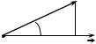
A vector line of a vector field F(M ) is a curve at whose every point M the direction of its tangent coincides with the direction of the vector of the field F at that point (Fig. 9.3).

For instance, the vector lines of a stationary velocity field of a fluid flow serve as trajectories of motion of the particles of the fluid (flow lines).

A collection of all vector lines of the field passing through any closed curve is called a vector tube.

Vector lines of the field

F (M ) = P(x, y, z)i + Q(x, y, z) j + R(x, y, z)k

may be determined from the following system of differential equations

along a tangent to the line AB at the point M. So as the vectors F(M) and dr are colinear, their coordinates are proportional, therefore the condition (9.5) is fulfilled.

9.3.2. Flux of a Vector Across a Surface

We consider the field of velocities v of fluid flow and take a surface σ in this field on which a definite side is chosen.

The flux of a vector across a surface is said to be a magnitude of fluid flowing across the surface for a unit of time.

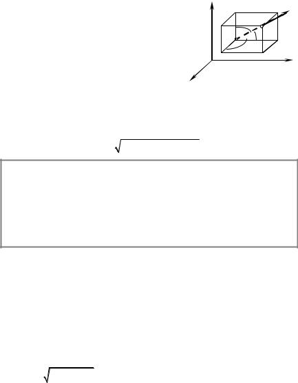
Let the velocity of flow be constant, and a surface σ be plane. In this case the fluid flow equals the volume of cylinder body (on Fig. 9.5 it is a sloping prism)

208

whose bases are parallel, and the length of every generatrix is v as for a unit of time every particle removes on the vector v , that is

F = Sh

prism numerically equal to the projection of the velocity v onto the unit normal vector n = {cos α, cosβ, cos γ} to the surface σ.

Thus,

F = (v n)S .

Now let the velocity v change continuously, and σ be a smooth surface. Let us choose a definite side of this surface. Let n = {cos α, cos β, cos γ } be a unit normal vector to the chosen side of the surface σ. Let us divide the surface σ on elementary parts σ1 , σ2 , ..., σn with areas Δσ1 , Δσ2 , ..., Δσn accordingly. We take the point Mk on every part σk and calculate the value of the velocity vector v at this point ( k = 1, 2, …, n ). Let us suppose that each elementary part is flat and the velocity vector is constant, equal to v(Mk ) (Fig. 9.6). For these

is a total quantity of fluid flowing across the whole surface for a unit of time.

The exact value of the quantity of fluid may be obtained, after passing to the limit on the left in the sum (9.6) provided every elementary surface compressed

to the point that is, for λ → 0, where λ = max dk is the greatest of diameters dk

1≤k ≤n

of elementary domain σk :

209

As F(M ) is the velocity vector field of a fluid flow the integral in (9.7) expresses the flux of fluid through the surface σ.

The flux of a vector field F(M ) across the surface σ is the integral of the

scalar product of the vector field by the unit normal vector to the surface taken over this surface:

F = ∫∫(F n)dσ .

σ

Other forms of representation of the vector field flux. 1. Taking into account properties of the dot product:

→

axes Ох, Оу and Оz accordingly, the flux of vector F can be represented in the following form

F = ∫∫(P cos α + Q cosβ + R cos γ )dσ ,

σ

or

The case of particular interest is that when the surface σ is closed and bounds a volume V. Then the flux is written down in the form of

The direction of the outer normal is taken as direction of the vector n . If the vector field F is the field of velocities of fluid flow, the value of the flux through

210