Добавил:

Upload Опубликованный материал нарушает ваши авторские права? Сообщите нам.

Вуз:

Национальный авиационный университет

Предмет:

[НЕСОРТИРОВАННОЕ]

Файл:

Higher Mathematics. Part 3

.pdf

Скачиваний:

201

Добавлен:

19.02.2016

Размер:

6.95 Mб

Скачать

☆

<<< < Предыдущая 1 2 3 4 5 6 7 8 9 10 11 12 13 14 15 16 17 18 19 20 2122 / 2422 23 24 > Следующая >>>

the closed surface equals a difference between the amounts of fluid flowing out the domain V and flowing into it for a unit of time. At the points of surface σ, where vector lines go out from the volume V, an outer normal forms an acute

angle with the vector F, consequently F n > 0 . At the points of surface σ, where vector lines enter the volume V, the outer normal forms an obtuse angle

with the vector F and F n > 0 .

If F > 0 the outflowing amount of fluid from the domain V exceeds the amount of fluid flowing into the domain. This means that there are sources inside the domain V generating the fluid.

If F < 0, the outflowing amount of fluid from the domain V is less than the

amount of fluid flowing into the domain. This means that there are sinks inside the domain V where the fluid disappears.

If F = 0, these amounts of fluid are in balance for the domain V. The

outflowing amount of fluid from the domain V is equal to the amount of fluid flowing into the domain. In this case there are neither sources nor sinks or they compensate each other.

9.3.3. Field Divergence.

Gauss — Ostrogradsky Formula in a Vector Form

Divergence of the vector field characterizes distribution and intensity of sources and sinks.

Let the vector field be given

F (M ) = P(x, y, z)i + Q(x, y, z) j + R(x, y, z)k ,

where R, Q and R are continuously differentiable functions in the corresponding domains.

Definition. The divergence of the vector field at the point M is said to be a number received by the formula

div F(M ) =	∂P	+	∂Q	+	∂R	,	(9.10)
	∂x		∂y		∂z

where partial derivatives are calculated at the point M.

Properties of divergence

1. If F is a constant vector, div F = 0.

2.div(C F) = C div F.

3.div(F1 + F 2 ) = div F1 + div F 2 .

4.If u is a scalar function, then div(uF) = u div F + F grad u.

Using notion of flux and divergence of the vector field, Gauss—Ostrog- radsky formula in a vector form can be rewritten as:

211

∫∫ (F n)dσ = ∫∫∫ divFdv

(9.11)

σV

Gauss—Ostrogradsky formula means that the flux of the vector F across the closed surface σ (in direction of the outer normal) equals a triple integral of the

divergence of the vector F over the volume V, bounded by this surface.

We can state another definition of the divergence, equivalent to the definition (9.10). By the theorem on the mean value for a triple integral in a domain V there

is such a point M0 where the equality is valid

∫∫ (F n)dσ = ∫∫∫ divF dv = V divF (M0 ) .

σV

Then the equality (9.11) can be written down in the form

∫∫ (F n)dσ = V divF (Mo ) .

The latter formula may be rewritten as

divF (Mo ) = 1 ∫∫ (F n)dσ . V σ

Let the surface σ be contracted to the point, that is, M0 → M , V → 0 and

divF (M ) = lim	1	∫∫ (F n)dσ .

V →0 V		σ

The divergence of the vector field F at a point M is the limit of the ratio of the flux of the vector field across a closed surface containing the point M to the volume of the domain bounded by this surface provided the surface is contracted to the point M.

If div F(M ) > 0 , the point M is a source, where the fluid flows out; if div F(M ) < 0 , the point M absorbes the fluid; and there are neither sources nor sinks inside the volume V, if div F = 0.

If div F = 0 at all points, then the vector field is called solenoidal or tubular.

9.3.4. Circulation of a Vector Field. Rotation of a Vector. Stokes’ Formula in a Vector Form

Let a continuous vector field be

F(M ) = P(x, y, z)i + Q(x, y, z) j + R(x, y, z)k and a closed oriented contour L be given in some domain D.

212

Let r = xi + yj + zk be a radius-vector of a point M lying on the contour L.

It is known, that the direction of the vector dr = dxi + dyj + dzk coincides the direction of the tangent τ in the positive direction round of the contour L (Fig. 9.7),

moreover | dr |= (dx)2 + (dy)2 + (dz)2 .

Definition. The circulation of a vector field F(M ) along a closed oriented contour L is said to be a line integral of the second type

C = ∫ F dr = ∫ Pdx +Qdy + Rdz.		(9.12)
L	L

Physical meaning of the circulation. If a closed oriented contour L is in a
field of force F , then the circulation is the work done by the force		F (M ) at
moving a material point along the contour L.

Definition. The rotation (or curl) of the vector field

F(M ) = P(x, y, z)i + Q(x, y, z) j + R(x, y, z)k

is called a vector

	∂R	−	∂Q	∂P		−	∂R		∂Q	−	∂P
rot F =	∂y	−	i +		∂z	−		j +	∂x	−	k.
	∂y		∂z		∂z		∂x		∂x		∂y

But it is easier to remember a symbolic form of the formula (9.13)

	i	j	k
rot F =	∂	∂	∂	.
	∂x	∂y	∂z

	P	Q	R

Stockes’ formula in a vector form looks as follows

∫ F dr = ∫∫ n rotFdσ.

(9.13)

(9.14)

that means that the circulation of a vector along a closed oriented contour L, bounding some surface σ, equals the flux of the curl through this surface (Fig. 9.8). Integration along the curve L goes in positive direction, that is, coherent with the direction of the normal to the selected side of the surface. If to look at the contour from the terminus of the normal, the contour is traced counterclockwise or in positive direction.

213

	z
	L	dr
		dr
	r	F(M)
	r	М(х, у, z)
	O	τ
	O	у
		у
	х

Fig. 9.7

		σ
	O	L
	O	у
		у

Fig. 9.8

Let us find out physical meaning of rotation.

Let a solid be rotated about the immovable axis l coinciding the axis Oz with an angular velocity of ώ. M (r) is a point of the body, where

r = xi + yj + zk .

The vector of the angular velocity is equal to ω = ωk , and the vector v of the linear velocity of the point M can be calculated as:

	i	j	k
v = ω × r =	0 0 ω			= − yωi + xωj.
	x	y	z

Using the definition of the rotation and found coordinates of the linear velocity (vector v ) we can receive

		i	j	k
rot v =		∂	∂	∂	= 2ωk = 2ω.
rot v =		∂x	∂y	∂z	= 2ωk = 2ω.
	− yω		xω	0

Thus, the rotation of the field of velocities of a solid rotating about an immovable axis is identical at all points of the field, parallel to the axis of rotation and equal to the doubled angular velocity of rotation.

9.3.5. Hamiltonian Operator.

Differential Operations of the First and Second Orders

All operations of vector analysis can be expressed by means of the Hamiltonian operator or a symbolic vector (it is read «nabla»), which is determined by the formula

= ∂∂x i + ∂∂y j + ∂∂z k.

214

Applying the well—known operations of multiplication of a vector by a scalar, scalar and vector multiplication of two vectors, we can obtain the differential operations of the first order:

1. u = ∂ i∂x

	∂
2. F =		i
2. F =	∂x	i
	∂x

		∂			∂
+			j +			k u =
+	∂y		j +	∂z		k u =
	∂y			∂z
		∂			∂		(Pi
+			j +			k
+		∂y	j +		∂z	k
		∂y			∂z

∂u i +	∂u	j +	∂u k = grad u .
∂x	∂y		∂z
+ Qj + Rk ) =			∂P	+	∂Q	+	∂R	= div F .
+ Qj + Rk ) =			∂x	+	∂y	+	∂z	= div F .

	i	j	k
3. × F =	∂	∂	∂	= rot F.
3. × F =	∂x	∂y	∂z	= rot F.
	P	Q	R

Using the well-known rules of vector algebra and rules of differentiation it is possible to obtain other formulas used in the field theory. In particular, a

directional derivative of the vector l = {cos α, cosβ, cos γ} may be rewritten as:

∂u = u l = (l u) = (l ) u.

∂l

In differential operations of the second order Hamiltonian operator is applied twice.

Let the scalar field u = u(x, y, z) be given. In this field the operator

generates the vector fieldu = grad u .

In the vector field two operations are defined:

а) u = div grad u.

b) × u = rot grad u.

Here the first operation has as a result a scalar field, and the second has a vector field.

Remark. Defined operations are similar to the operations of scalar and vector products formed by two vectors.

Let the vector field F = Pi + Qj + Rk be given. Then the operator generates:

а) a scalar field of div F where the operator generates the vector field( F) = grad div F ;

b) a vector field rot F where the operator can form:

a scalar field ( × F) = div rot F ; a vector field × ( × F) = rot rot F .

215

Thus, there are five differential operations of the second order:

div grad u ,

rot grad u ,

grad div F , div rot F ,

rot rot F

Let us consider these operations.

∂2

1. div grad u = ( u) = ( )u =

∂x

∂y

∂z

∂2u

u .

∂x2

∂y2

∂z

Here = =

∂2

is Laplace’s operator.

∂x2

∂z2

∂y2

An operator

(delta) plays an important role in mathematical physics.The

equation u = 0 is called Laplace’s equation.

A scalar field u = u(x, y, z), satisfying Laplace’s equation, is called harmonic.

2. rot grad u = × ( u) = ( × )u = 0 so as a dot product of two equal (or

collinear) vectors equals zero (zero-vector). Thus, the field of gradient is irrotational.

3. div rot F = ( × F) = 0 so as the mixed product of three vectors, two of which are identical equals zero.Thus, the field of rotation is solenoidal.

Operations grad div F and rot rot F are applied rarely, therefore we do not consider them.

9.3.6. Some Properties of Vector Fields. Solenoidal Field

A vector field F is called solenoidal, if its divergence equals zero at all points, i.e. div F = 0.

Properties of the solenoidal field

1. In the solenoidal field F the flux of a vector across any closed surface equals zero. Thus, the solenoidal field has neither sources nor sinks.

2. A solenoidal field is a field of rotation of some vector field, that is, if div F = 0, there exists such field B that B = div F = 0. The vector B is called a vector potential of the field F .

216

3. In the solenoidal field of a vector tube (a set of constant value.

F the flux of a vector across the transversal section vector lines passing through a border L) has the

Potential Field

A vector field F is called potential, if there exists such a function u(M )

that
grad u = F,	(9.15)

i.e. the vector field is a gradient of some scalar field.

The vector equality (9.15) is equivalent to three scalar equalities:

∂u	= P(x, y, z),	∂u	= Q(x, y, z),	∂u	= R(x, y, z) .
∂x		∂y		∂z

There is another equivalent definition of a potential field.

A vector field F is called potential, if for all points of the field

rot F = 0.

Let us prove that if a vector field is a gradient of some scalar field, that is,

grad u = F then rot F = 0. We have

rot F = rot grad u = rot

∂u

i +

∂u

j +

∂u

∂x

∂y

∂z

∂2u

∂

∂2u

−

i −

−

j +

−

k = 0.

∂x ∂y ∂z

∂y∂z

∂x∂z

∂z∂y

∂z∂x

∂x∂y ∂y∂x

∂u

∂x

∂y

∂z

Properties of the potential field

1. Circulation of the potential field F along any closed contour in this field equals zero.

2. In the potential field F a line integral ∫ Pdx + Qdy + Rdz along an arbitrary

curve L does not depend on the form of the curve but only on the initial and terminal points of the curve L.

217

The potential of the vector field can be defined by the formula

			( x, y, z)	x
	u(x, y,	z) =	∫	Pdx + Qdy + Rdz = ∫ P(x, y0 , z0 )dx +
			( x0 , y0 , z0 )	x0	(9.16)
			y	z	(9.16)
			+ ∫ Q(x, y, z0 )dy + ∫ Q(x, y, z)dz,
			y0	z0
where (x0 , y0 , z0 )		are coordinates of a fixed point, (x, y, z) are co-ordinates of

an arbitrary point. We should note that a potential is determined by accuracy to the constant, because of grad(u + C) = grad u.

Harmonic Field

A vector field F is called harmonic, if it is simultaneously potential and solenoidal, that is, if

rot F = 0 and div F = 0.

The field of linear velocities of stationary irrotational flow of fluid is an example of a harmonic field provided it has neither sources nor sinks inside it.

The condition of potentiality of the field means that the vector field can be

represented as	F = grad u , where u(x, y,	z) is the field potential. At the same
time the field	is solenoidal, therefore	div F = div grad u = u = 0 , in other

words, the potential of this field is a harmonic function, that is, the solution of Laplace’s equation

∂2u + ∂2u + ∂2u = 0. ∂x2 ∂y2 ∂z2

Micromodule 9

EXAMPLES OF PROBLEM SOLUTIONS

Example 1. Find the greatest rate of increase of the scalar field u = x2 +2y2 +4z2 at the point M (−1; 2; 2) .

Solution. The value of the greatest rate of increase of the scalar field u at the

given point equals the modulus of a gradient of the field calculated at this point (see (9.4)). We have

∂u(M )

= −

∂u

2 y

∂x

x2 + 2 y2 + 4z2

∂y

x2 + 2 y2 + 4z2

218

∂u

∂z

x2 + 2y2 + 4z2

grad u

4 2

8 2

−

+ 16 + 64 =

Example 2. Find the divergence and rotation of the vector field

F = x2i + y2 j − z2 k.

Solution. We have

P = x2 , Q = y2 , R = − z2 ;

∂P

= 2x,

∂Q

= 2 y, ∂R

= −2z.

∂x

∂y

∂z

Then by the formula (9.10) we obtain

div F = 2x + 2 y − 2z = 2(x + y − z) .

As ∂R =

∂Q =

∂P

∂R

∂Q

= ∂P = 0, in

accordance

with the formula

∂y

∂z

∂x

∂y

(9.13) rot F = 0, that means the given field is irrotational.

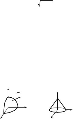
Example 3. Calculate the flux of the vector field

F = xi + yj + zk across the

part of the sphere x2 + y2 + z2

= 1 placed in the first octant, in direction of the

outer normal (Fig. 9.9).

F n = (xi + yj + zk ) (xi + yj + zk ) = x2 + y2 + z2 .

Solution. The first method. As a flux of the vector field across the given surface is expressed by a surface integral (9.8), where R = x, Q = y, R = z, the

interal ∫∫ xdydz + ydzdx + zdxdy should be calculated. It may be considered as a

sum of three integrals F = I1 + I2 + I3 . For the calculation of I1 we have to project the given surface onto the plane Oyz. We obtain a quarter of a circle

Dyz : y2 + z2 ≤ 1,	0 ≤ y ≤ 1,	0 ≤ z ≤ 1.	The equation of the sphere can be solved
relative to the variable x : x =		1− y2 − z2 . Then
			π
I1 = ∫∫ xdydz = ∫∫			2	1		π .
I1 = ∫∫ xdydz = ∫∫		1− y2 − z	2 dydz = ∫ dϕ∫		1− ρ2 ρdρ =	π .
σ	Dyz		0	0		6
σ	Dyz		0	0
						219

Taking into account symmetry of the vector field and surface σ we reach to

the conclusion, that I2 = I3	= I1 = π , therefore F = I1	+ I2 + I3 = 3	π	=	π .
	6		6		2
The second method. So as for points of the sphere		n = xi + yj + zk			is a unit
normal vector to the sphere	x2 + y2 + z2 = 1 (prove it yourself)
F n = (xi + yj + zk ) (xi + yj + zk ) = x2 + y2 + z2 ,
and
F = ∫∫(F n)dσ = ∫∫(x2 + y2 + z2 )dσ = ∫∫ dσ.
σ	σ	σ

Thus, the flux of the field

F equals the area of the given surface, that is, ⅛

of the sphere, that is, F =

4π 1

= 2 .

Example 4. Calculate the flux of the vector field F = x2 i + y2 j + k

across

the complete surface of the cone

z = 1−

x2 + y2 bounded by the plane

z = 0

(Fig. 9.10), using Gauss—Ostrogradsky formula.

Solution. Let us find the divergence of the vector field:

div F =

∂

(x2 ) +

∂

( y2 ) +

∂

(1) = 2(x + y).

∂x

∂y

∂z

Using formulas (9.9) and (9.11), we calculate the flux of the given field:

			F = ∫∫∫		divFdxdydz = 2∫∫∫ (x + y)dxdydz =
			G					G
2π		1	1−ρ			2π		1	((cos ϕ + sin ϕ)ρ z)				1− ρ ρdρ =
2π		1	1−ρ			2π		1
= 2 ∫ dϕ∫ρdρ ∫ (ρ cos ϕ + ρ sin ϕ)dz = ∫ dϕ∫
	0	0	0				0	0					0
	0	0	0				0	0					0
	2π			1			2π		ρ3			ρ4		1
	2π			1			2π		ρ3			ρ4		1
=	∫	(cos ϕ + sin ϕ)dϕ		∫	ρ2	(1− ρ)dρ =	∫				−			dϕ =
=		(cos ϕ + sin ϕ)dϕ			ρ2	(1− ρ)dρ =		(cos ϕ + sin ϕ)		3	−	4		dϕ =
	0			0			0							0
	0			0			0							0

			1	2π
	=		1	∫ (cos ϕ + sin ϕ)dϕ = 0.
	=	12		∫ (cos ϕ + sin ϕ)dϕ = 0.
	z	12		0
				0
				z
	1		n	z
	1		n
		1		y	y
	1				y
x	1			x
x				x
	Fig. 9.9			Fig. 9.10

220

<<< < Предыдущая 1 2 3 4 5 6 7 8 9 10 11 12 13 14 15 16 17 18 19 20 2122 / 2422 23 24 > Следующая >>>

Соседние файлы в предмете [НЕСОРТИРОВАННОЕ]

#
19.02.20166.14 Mб380gr.doc
#
30.04.2019424.45 Кб11Graphics software.doc
#
05.09.2019478.78 Кб6gtfnmТ.docx
#
15.08.2019637.53 Кб4Gulenko.docx
#
12.11.2018765.44 Кб6Hagakure_-_Sokrytoe_v_listve.doc
#
19.02.20166.95 Mб201Higher Mathematics. Part 3.pdf
#
19.02.20166.63 Mб1052Higher_Mathematics_Part_1.pdf
#
19.02.20169 Mб95Higher_Mathematics_Part_1.pdf
#
19.02.20167.48 Mб408Higher_Mathematics_Part_2.pdf
#
19.02.20169.73 Mб45Higher_Mathematics_Part_2.pdf
#
19.02.20167.31 Mб123Higher_Mathematics_Part_2.pdf