XRF

Principles of X-ray Fluorescence

Table of contents

Principles of X-ray Fluorescence

Principles of X-ray Fluorescence

1.Introduction

This document gives a general introduction to X-Ray Fluorescence (XRF) spectrometry and XRF analysis. It explains simply how a spectrometer works and how XRF analysis is done. It is intended for people new to the field of XRF analysis. Difficult mathematical equations are avoided and the document requires only a basic knowledge of mathematics and physics.

The document is not dedicated to one specific type of spectrometer or one application area, but aims to give a global overview of the main spectrometer types and applications.

Section 2 briefly explains XRF and its benefits. Section 3 explains the physics of XRF, and section 4 describes how this physics is applied to spectrometers and their components. Section 5 explains how an XRF analysis is done. It describes the process of sample taking, measuring the sample and calculating the composition from the measurement results. Finally, section Error! Reference source not found. gives a list of related literature for further information on XRF analysis.

Principles of X-ray Fluorescence

2.What is XRF

XRF is an analytical method to determine the chemical composition of all kinds of materials. The materials can be in solid, liquid, powder, filtered or other form. XRF can also sometimes be used to determine the thickness and composition of layers and coatings.

The method is fast, accurate and non-destructive, and usually requires only a minimum of sample preparation. Applications are very broad and include the metal, cement, oil, polymer, plastic and food industries, along with mining, mineralogy and geology, and environmental analysis of water and waste materials. XRF is also a very useful analysis technique for research and pharmacy.

Spectrometer systems can be divided into two main groups: energy dispersive systems (EDXRF) and wavelength dispersive systems (WD-XRF), explained in more detail later. The elements that can be analyzed and their detection levels mainly depend on the spectrometer system used. The elemental range for ED-XRF goes from Sodium to Uranium (Na to U). For WD-XRF it is even wider, from Beryllium to Uranium (Be to U). The concentration range goes from (sub) ppm levels to 100%. Generally speaking, the elements with high atomic numbers have better detection limits than the lighter elements.

The precision and reproducibility of XRF analysis is very high. Very accurate results are possible when good standards are available, but also for applications were no specific standards can be found.

The measurement time depends on the number of elements to be determined and the required accuracy, and varies between seconds and 30 minutes. The analysis time after the measurement is only a few seconds.

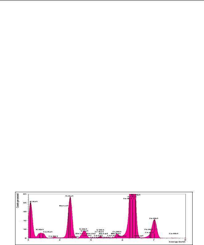
Figure 1 shows a typical spectrum of a soil sample measured with ED-XRF – the peak profiles are clearly visible. The positions of the peaks determine the elements present in the sample, while the heights of the peaks determine the concentrations.

Figure 1 Typical spectrum of a soil sample measured with an ED-XRF spectrometer.

Principles of X-ray Fluorescence

3.Basics of XRF

In XRF, x-rays produced by a source irradiate a sample. In most cases the source is an x-ray tube. The elements present in the sample will emit fluorescent x-ray radiation with discrete energies (equivalent to color for optical light) that are characteristic for these elements. A different energy is equivalent to a different color. By measuring the energies (determining the colors) of the radiation emitted by the sample it is possible to determine which elements are present. This step is called Qualitative Analysis. By measuring the intensities of the emitted energies (colors) it is possible to determine how much of each element is present in the sample. This step is called Quantitative Analysis.

3.1.What are x-rays

X-rays can be seen as ElectroMagnetic (EM) waves with their associated wavelengths, or as beams of photons with associated energies. Both views are correct, but one or the other is easier to understand depending on the phenomena to be explained. Other electromagnetic waves include light, radio waves and γ-rays. Figure 2 shows that x-rays have wavelengths and energies between γ-rays and ultra violet light. The wavelengths of x-rays are in the range from 0.01 to 10 nm, which corresponds to energies in the range from 0.125 to 125 keV. The wavelength of x-rays is inversely proportional to its energy, according to E* λ =hc. E is the energy in keV and λ the wavelength in nm. The term hc is the product of Planck’s constant and the velocity of light and has, for the using keV and nm as units, a constant value of 1.23985.

γ-raysX-raysUVVisual

Wavelength 0.001 0.01 0.1 1.0 10.0 100 200 nm

Figure 2 x-rays and other electromagnetic radiation.

3.2.Interaction of x-rays with matter.

There are three main interactions of x-rays with matter: Fluorescence, Compton Scatter and Rayleigh Scatter. If x-rays fall on material a fraction will pass through the sample, a fraction is absorbed into the sample and produces fluorescent radiation, and a fraction is scattered back. Scattering can occur with loss of energy and without loss of energy. The first is called Compton scatter and the second Rayleigh scatter. The fluorescence and the scatter depend on the thickness (d), density (ρ) and composition of the material and on the energy of the x-rays. The next sections will describe the production of fluorescent radiation and scatter.

d

Figure 3 Three main interactions of x-rays with matter.

Principles of X-ray Fluorescence

3.3.Production of characteristic fluorescent radiation.

The classical model of an atom is a nucleus with positively charged protons and non-charged neutrons, surrounded by electrons grouped in shells or orbitals. The innermost shell is called the K-shell, followed by L-shells, M-shells etc travelling outwards. The L-shell has 3 sub-shells

called LI, LII and LIII. The M-shell has 5 sub-shells MI, MII, MIII, MIV and MV. The K-shell can contain 2 electrons, the L-shell 8 and the M-shell 18. The energy an electron has depends on

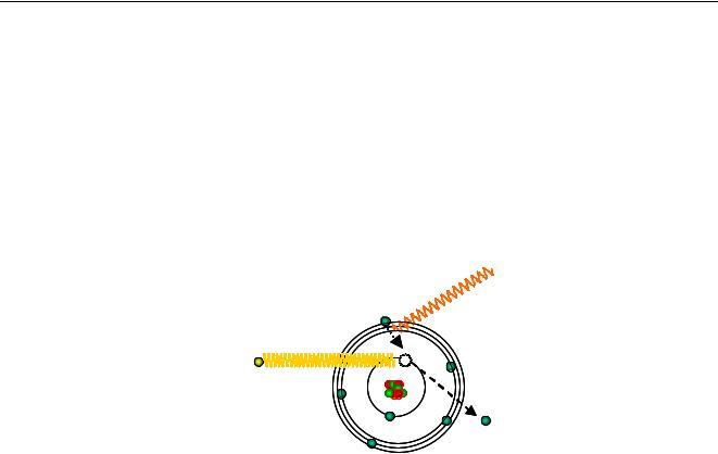
the shell it is in, and on the element to which it belongs. Irradiating an atom, particles like X- ray photons and electrons with sufficient energy can expel an electron from the atom (Figure 4).

Characteristic photon

Incoming photon

Expelled electron

Figure 4 Production of characteristic radiation.

This produces a hole in a shell, in the example a hole in the K-shell, putting the atom in an unstable situation with a higher energy. The atom wants to restore the original configuration, and this is done by transferring an electron from an outer shell e.g. the L-shell to the hole in the K-shell. An L-shell electron has a higher energy than a K-shell electron, and when an L-shell electron is transferred to the K-shell, the energy surplus is emitted as x-rays. In a spectrum, this is seen as a line. The energy of the emitted x-rays depends on the difference in energy of the shell with the initial hole and the energy of the electron that fills the hole (in the example, the difference between the energy of the K and the L shell). Each atom has its specific energy levels, so the emitted radiation is characteristic for that atom. An atom emits more than just one energy (or line), because different holes can be produced and different electrons can fill up these holes. Because the energy levels are characteristic for an element, the emitted x-rays are also characteristic for the element and are more or less a fingerprint.

To expel an electron from an atom, the x-rays must have a higher energy than the binding energy of the electron. If an electron is expelled, the incoming radiation is absorbed and the higher the absorption the higher the fluorescence. If on the other hand the energy is too high, many photons will ‘pass’ the atom and only a few electrons will be removed. Figure 5 shows that high energies are hardly absorbed and produce low fluorescence. If the energy is lower and comes closer to the binding energy of the K-shell electrons, more and more radiation is absorbed. The highest yield is reached when the energy of the photon is just above the binding energy of the electron to be expelled. If the energy becomes lower then the binding energy, a jump or edge can be seen: the energy is too low to expel electrons from that shell, but is too high to expel electrons from the lower energetic shells. The figures show the K edge corresponding to the K shell, and three L edges corresponding with the LI, LII and LIII shells.

Principles of X-ray Fluorescence

Energy keV

Figure 5 Absorption versus energy

The ability to expel electrons from an atom depends on the atom involved. In general it is easier to expel an electron from heavy elements than from light elements. Figure 6 shows the fluorescence yield for K and L electrons as a function of the atomic number Z. The fluorescence yield is the ratio of the vacancies produced and the required number of incoming photons. The Figure clearly shows that the yield is low for the very light elements, explaining why it is so difficult to measure these elements.

Figure 6 Fluorescence yield for K and L electrons.

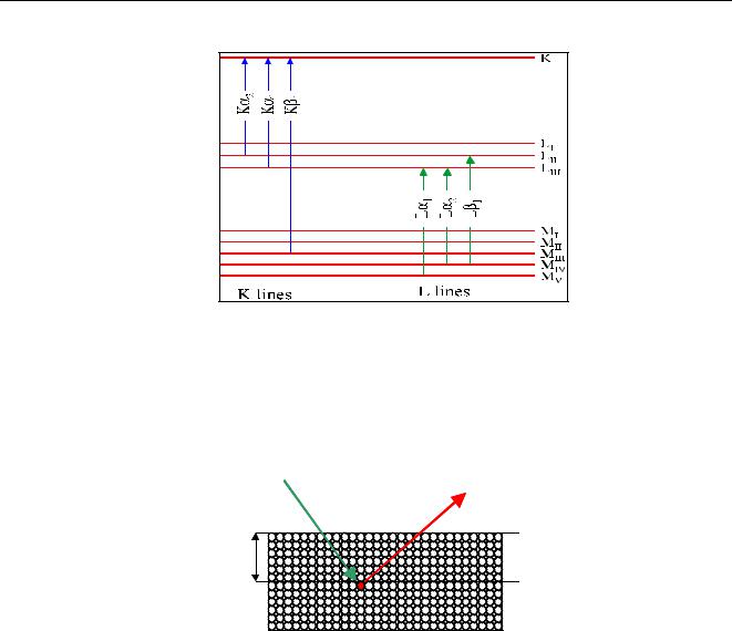
There are several ways to indicate different lines. The Siegbahn and IUPAC notations are the two most found in literature. The Siegbahn notation indicates a line by the symbol of an element followed by the name of the shell where the initial hole is and a Greek letter (α,β,γ etc) indicating the relative intensity of a line. E.g. Fe-Kα, is the strongest Iron line due to an expelled K electron. The Siegbahn notation however does not give tell from which shell the electron comes that fills the hole. In the IUPAC notation, a line is indicated by the element and the shell where the initial hole was, followed by the shell where the electron comes from that fills up this hole. For example, Cr-KLIII is Chromium radiation due to a hole produced in the K- shell filled by an electron in the LIII shell. Generally, K-lines are more intense than L-lines which are more intense than M-lines and so on. Quantum mechanics teaches that not all transitions are allowed, for instance a transition from the LI to the K shell. Figure 7 gives an overview of the most important lines with their transitions.

Principles of X-ray Fluorescence

Figure 7 Major lines and their transitions

3.4.Absorption and enhancement effects.

To reach the atoms inside the sample the x-rays have to pass the layer above it, and this layer will absorb a part of the incoming radiation. The characteristic radiation produced also has to pass this layer to leave the sample, and again part of the radiation will be absorbed.

Figure 8 Absorption of incoming and fluorescent x-rays

The magnitude of the absorption depends on the energy of the radiation, the path length d of the atoms that have to be passed, and the density of the sample. The absorption increases as the path length, density and atomic number of the elements in the layer increases, and as the energy of the radiation decreases. The absorption can be so high that elements deeper in the sample are not reached by the incoming radiation or the characteristic radiation can no longer leave the sample. This means that only elements close to the surface will be measured.

The incoming radiation is x-rays, and the characteristic radiation emitted by the atoms in the sample itself are also x-rays. These fluorescent x-rays are sometimes able to expel electrons from other elements in the sample. This, as with the x-rays coming from the source, results in fluorescent radiation. The characteristic radiation produced directly by the x-rays coming from the source is called primary fluorescence, while that produced in the sample by primary fluorescence of other atoms is called secondary fluorescence.

Principles of X-ray Fluorescence

Primary

Figure 9 Primary and secondary fluorescence

A spectrometer will measure the sum of the primary and secondary fluorescence, and it is impossible to distinguish between both contributions. The contribution of secondary fluorescence to the characteristic radiation can be significant (in the order of 20%). Similarly, tertiary and even higher order radiation can occur. In almost all practical situations these are negligible, but in very specific cases can reach values of 3%.

3.5.Absorption and analysis depths.

As the sample gets thicker and thicker, more and more radiation is absorbed. Finally radiation produced in the deeper layers of the sample is no longer able to leave the sample. When this limit is reached depends on the material and on the energy of the radiation.

Table 1 gives the approximate analysis depth in various materials for three lines with different energies. Mg Kα has an energy of 1.25 keV, Cr Kα 5.41 keV and Sn Kα 25.19 keV.

Table 1 Analysis depth in µm (unless indicated otherwise) for three different lines and various materials.

When a sample is measured, only the atoms within the analysis depth are analyzed. If samples and standards with various thicknesses are analyzed, the thickness has to be taken into account.

3.6.Rayleigh and Compton scatter.

A part of the incoming x-rays is scattered (reflected) by the sample instead of producing characteristic radiation. Scatter happens when a photon hits an electron and is bounced away. The photon loses a fraction of its energy, which is taken over by the electron as shown in Figure 10. It can be compared with one billiard ball colliding with another. After the collision, the first ball lost a part of its energy to the ball that was hit. The fraction that is lost depends on the angle at which the electron (ball) was hit. This type of scatter is called Compton or incoherent scatter.