XRF

Principles of X-ray Fluorescence

Figure 36 Two overlapping peaks and their sum

Deconvolution is used to determine the area of the individual profiles. The measured spectrum is fitted to theoretical profiles. The area of these profiles is changed, but keeping the shape fixed, until the sum of all the profiles gives the best fit with the measured spectrum. One way would be to try all possible combinations of profiles, but this would take a long time to find the best fit. Instead, a mathematical method called Least Square Fitting finds the best fitting peak profiles, but this can still be time consuming. Theoretical calculations are also used to find the best fit. From theory, it is possible to calculate the ratios between groups of line intensities. This reduces the number of free parameters, finding the best fit more quickly.

The background has to be taken into account when fitting the peak profiles. First stripping the background, and fitting the profiles to the resulting net spectrum can do this. It is also possible to fit background and peak profiles to the measured spectrum in one process.

Mathematically it is formulated as find the heights heightp and widths widthp of all the peak profiles described by the function Pc, that minimizes the following sum:

In this equation Rem is the measured intensity in energy e, Be the background at energie e.

Principles of X-ray Fluorescence

5.4.Qualitative Analysis in WD-XRF

5.4.1. Peak Search and Peak Match

As with ED-XRF, Peak Search and Peak Match are used to discover which elements are present in the sample. Once again, Peak Search finds the peaks, and Peak Match determines the associated elements by referring to a database.

5.4.2. Measuring peak height and background subtraction.

In WD-XRF it is common practice to measure the intensity at the peak of a line and on a few background positions close to the peak. The positions must be chosen carefully and must be free of other peaks. The background under the peak is determined by interpolating the intensities measured at the background positions.

Figure 37 Determination of net intensity

5.4.3. Line overlap correction

Figure 38 shows two overlapping lines and their sum. Here, the height of the peak cannot be determined as the raw intensity minus the background.

Figure 38 Two overlapping peaks and their sum

The intensity measured at position 1 is the sum of the net height of peak 1 and a factor of peak 2, and vice versa. Mathematically this can be written as

Principles of X-ray Fluorescence

This is a set of 2 linear equations, and the net intensities of both peaks can be calculated if the factors f12 and f21 are known. These two factors can be determined using a reference sample that contains only element 1, and another containing only element 2. For element 2, such a sample will give a spectrum like that in Figure 39.

Figure 39 Determination of overlap factor

The fraction of peak 2 that overlaps with peak 1 is calculated as f12 = R2,1 . The overlap

R2

factor f21 of line 1 on line 2 can be determined in the same way.

5.5.Counting statistics and detection limits

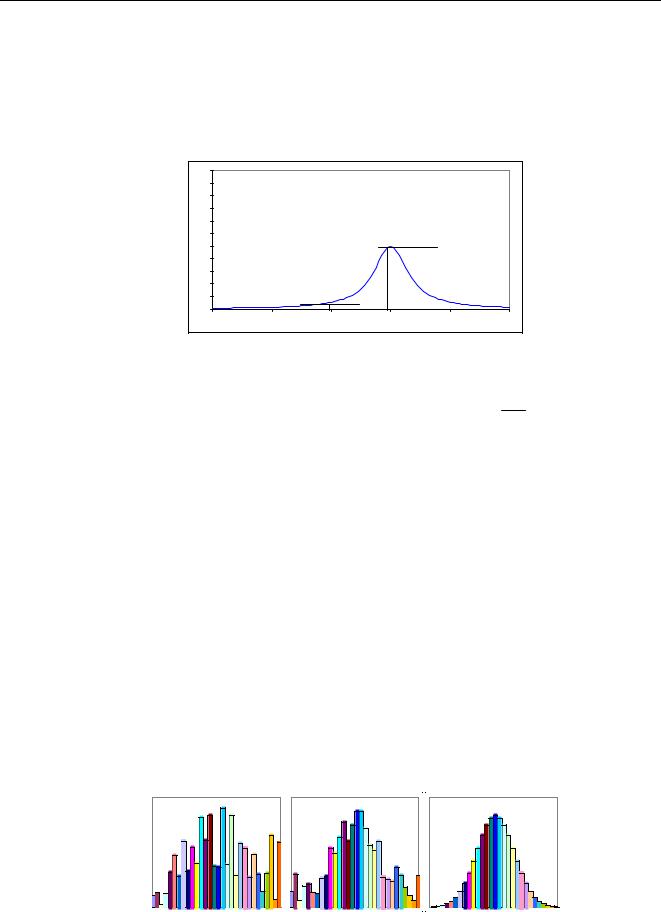
The detector counts incoming photons, which is similar to counting raindrops. When it rains, the number of drops falling into a bucket in a second is not always exactly the same. Measuring for a longer time and calculating the average per second gives a more accurate result. If it is raining heavily, only a short time is required to give an accurate number of drops per second, but a longer time is needed if it is only raining lightly.

Raindrops have different sizes and counting all the drops with a specific size is equivalent to measuring the intensity of the radiation of one particular element in the complete spectrum. Telling whether there are more drops with one size than those with another size means that sufficient drops have to be counted. A histogram of the counted raindrops would look like Figure 40. The height of a bar corresponds to the number of drops counted having a specific size. The leftmost picture is the result after a short time, the middle after counting for longer and the rightmost after counting for a very long time. The longer the count, the clearer it becomes that the number of drops is not the same for each size.

Figure 40 Number of raindrops counted per second

Principles of X-ray Fluorescence

Now back to x-rays. To detect a peak of an element, it must be significantly above the noise (variation) in the background. The noise depends on the number of x-ray photons counted. The lower the number of photons counted, the higher the noise. The analysis is commonly done on the number of photons counted per second, but as above the noise depends on the total number of photons counted. By measuring for a longer period, it is possible to collect more photons and hence reduce the noise.

Figure 41 Spectra measured over different times

Figure 41 shows three scans of the same material, but with different measurement times. In the first spectrum it is difficult to determine the peaks and their heights. In the second, the peaks are more prominent and in the third they can be clearly seen and their net height can be determined accurately. A commonly accepted definition for the detection limit is that the net intensity of a peak must be 3 times higher than the standard deviation of the background noise. The standard deviation of the background noise equals the square root of the intensity (in counts), so elements are said to be detectable if

N p ≥ 3 where Np is the number of counts measured on the peak and Nb the number of counts

Nb

measured on the background. For low backgrounds, low line intensities are sufficient to fulfil the requirement, so a low background gives low detection limits. 3D optics is used to reduce the background.

5.6.Quantitative Analysis in ED-XRF and WD-XRF

Quantitative analysis is basically the same for ED-XRF and WD-XRF. The only difference is that in ED-XRF the area of a peak gives the intensity, while in WD-XRF the height of a peak gives the intensity. The exact same mathematical methods can used to calculate the composition of samples.

In the Quantitative Analysis, the net intensities are converted into concentrations. The usual procedure is to calibrate the spectrometer by measuring one or more reference materials. The calibration determines the relationship between the concentrations of elements and the intensity of the fluorescent lines of those elements. Unknown concentrations can be determined once the relationship is known. The intensities of the elements with unknown concentration are measured, with the corresponding concentration being determined from the calibration

5.6.1. Matrix effects and Matrix Correction Models

Ideally, the intensity of an analytical line is linearly proportional to the concentration of the analyte and, across a limited range, this is the case. However, the intensity of an analytical line does not only depend on the concentration of the originating element. It also depends on the

Principles of X-ray Fluorescence

presence and concentrations of the other elements. These other elements can lead to attenuation or to enhancement.

Figure 42 (left) illustrates the absorption effect. To reach atoms inside a specimen, the x-rays from the source must first pass the atoms that are above them, and the fluorescence from the atoms must also similarly pass these atoms. These overlying atoms will absorb a part of the incoming radiation and a part of the fluorescent radiation. The absorption depends on which elements are present and on their concentrations. In general, heavy elements absorb more than light elements.

Figure 42 Absorption and enhancement effects

Figure 42 (right) shows the enhancement effect. An element is excited by the incoming radiation but in some cases also by the fluorescence of other elements. Whether or not this occurs and how large the effect is depends on the elements and their concentrations.

Across a limited range, the curve can be approximated by a straight line given by C=D+E*R, where D and E are determined by linear regression. This line can only be used for samples that are similar to the standards used, and across a limited range. Normally, it definitely cannot be used for other types of samples. A better fit and a wider range comes from adding more terms like C=D+E*R+F*R*R, but the range will still be limited and only applicable to samples similar to the standards.

Figure 43 Calibration with linear and parabolic fit

Matrix correction models use terms to correct for the absorption and enhancement effects of the other elements. This is done in various ways, but they all in one way or another use the relation

Ci = Di + Ei Ri Mi

or

Ci = (Di + Ei Ri ) Mi

Principles of X-ray Fluorescence

This document discusses the first relation, but the method is also applicable to the second relation. M is the matrix correction factor, and the difference between the models lies in the way they define and calculate M.

5.6.1.1. Influence of Coefficient matrix correction models

These models have the shape

Ci = Di + Ei Ri [1+ corrections]

The corrections are numeric values depending on the concentrations and/or intensities of the matrix elements. Many people have suggested ways to define and model the corrections, and models are commonly named after the person(s) who proposed it.

A commonly used method has been proposed by and named after De Jongh, and is given by:

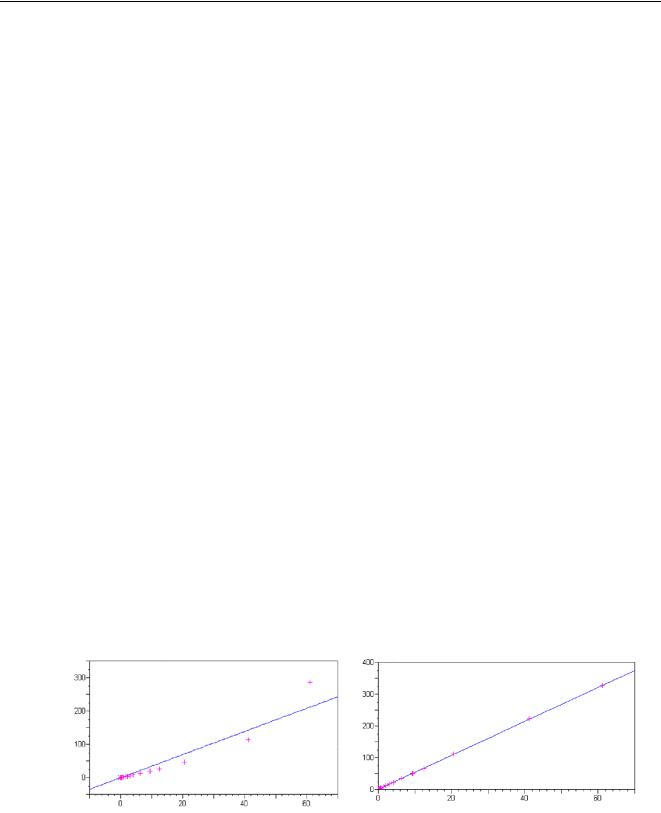
The α’s are numeric values that give how much element j attenuates or enhances the intensity of the analyte i. Because the sum of all concentrations in a specimen equals 1, one element can be eliminated, indicated by j≠e. The element being eliminated is often the major component like Fe in steel or Cu in copper based alloys. The values of the α’s are calculated by theory using ‘Fundamental Parameters’. (see also section 5.6.1.2). After the α’s have been calculated, at least two standards are required to calculate D and E (only one if D is fixed). Instead of calculating the values of the α’s by theory, it is possible to calculate them by regression. Then, a set of different standards is measured and the values of D, E and the α’s are calculated. The equations can be extended with additional correction factors leading to more comprehensive models. The left picture of Figure 44 shows a calibration of Ni in steel without any corrections and the right picture shows the same if corrections are applied.

Figure 44 Calibration of Ni without correction and with alpha corrections

5.6.1.2. Fundamental Parameter (FP) matrix correction models

Fundamental Parameter models are based on the physics of x-rays. In the 1950s, Sherman derived the mathematical equations that describe the relationship between the intensity of an element and the composition of a sample. This equation contains many physical constants and

Principles of X-ray Fluorescence

parameters that are called Fundamental Parameters. The Sherman equation is used to calculate the values of the matrix correction M fully by theory and the model becomes:

Ci = Di + Ei Ri Mi

At least two standards are required to calculate D and E, or just one if only E has to be calculated. M is calculated for each individual standard, and the factors D and E are determined for all elements.

The matrix factors M can only be calculated accurately if the full matrix is known, because all absorption and enhancements have to be taken into account. The calculations are quite involved and require a powerful computer which, until recently, made these models unsuited for routine operations. Because FP accounts for all effects, it can be used over virtually the full concentration range and for all types of samples as long as the majors are known.Figure 45 shows the results using the same FP calibration for samples with a very wide concentration range.

Certified (%)

Figure 45 Results of FP analysis for various samples.

5.6.1.3. Compton matrix correction models

The Compton method is an empirical one. The intensity of a Compton scattered line depends on the composition of the sample. Light elements give high Compton scatter, and heavy elements low Compton scatter, which is used to compensate for the influence of the matrix. The model is.

Ci = Di + Ei Ri

Rc

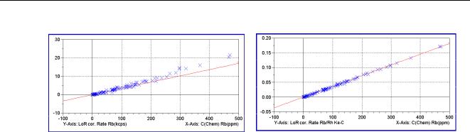
The Compton line can be a scattered tube line, or a line originating from a secondary target if 3D optics is used. The righr picture of Figure 46 shows a calibration without any corrections and the right picture shows the same if Compton correction is used.

Principles of X-ray Fluorescence

Figure 46 Calibration without and with Compton Correction

5.6.2. Line overlap correction

Sections 5.3.2 and 5.4.3 explained how overlapping lines were resolved, by subtracting a fraction of the overlapping peak from the peak of interest. The fractions were determined by measuring dedicated standards. Another method is to determine the overlap factors by regression. The calibration model is extended with terms that describe the line overlap.

The overlap factors fij are determined by regression. The problem with this equation is that it can be non-linear, which makes it difficult to calculate the factors. If the calibration is limited to a small range, and when the variation in M is small, it can be approximated by

Ci = Di − ∑ fij Rj + Ei Ri Mi

overlapping lines j

This is a linear equation, and it is mathematically easy to calculate the overlap factors fij and the other calibration parameters simultaneously.

These methods require that the overlapping intensities be measured. In ED-XRF this is not a problem because the whole spectrum is generally measured. In WD-XRF, often only the lines of the elements of interest are measured and not the overlapping lines. The intensity of the overlapping lines is, over a limited range, proportional to the concentration of the originating element. The following equation can therefore be used.

Ci = Di − ∑ fij Cj + Ei Ri Mi

overlapping lines j

5.6.3. Drift correction

The stability and reproducibility of spectrometers is high, but long-term drift is unavoidable. The tube and the detector degrade over time and the response of the other components can also change over time. Because of this drift, a calibration is not valid after a certain period of time. Calibrating anew can be time consuming, and an alternative is to apply drift correction. Here, one or more special monitor samples are measured, and the relative change in intensity of the monitor samples is also applied to the samples being analyzed.

Principles of X-ray Fluorescence

5.6.4. Thin samples.

Thin samples require special treatment. For thick samples, the intensity corrected for matrix effects is linearly proportional to the concentration and does not depend on the thickness of the sample. This is because only radiation coming from a layer close to the surface can leave the detector and reach the detector. Radiation coming from deeper layers is not detected, and making the sample thicker will have no effect on the measured intensity.

This is different for thin samples. As long as the radiation from the bottom of the sample can still pass through the sample and reach the detector, it will affect the measured intensity. If the measured intensity for thin samples is lower than the intensity of a standard, it is not possible to tell whether the concentration of the analyte is lower or whether the sample is thinner than the standard.

If the thickness of the sample is known, it can be taken into account and it again becomes possible to calculate the concentration of the analyte. This requires complex mathematics, and is beyond the scope of this document.

5.7.Analysis methods

Analysis uses the same equations used for the calibration. In the calibration, the D, E and correction factors are the parameters that have to be determined. The concentrations are known because standards with known composition were used. In the analysis, the opposite is true. The D, E and correction factors are (assumed to be) known and the concentrations are the unknowns that have to be determined. Often this is done by iterative methods.

The process starts with an initial guess at the concentrations, and these concentrations are substituted in the right hand side of the equations. This gives new values for the concentrations that are substituted in the right hand sides, again giving new values for the concentrations. This process is repeated until the concentrations converge to limiting values. The result of the final iterations is assumed to be the composition of the sample.

C1 = D1 + E1 R1 M1(C1..Cn , R1..Rn ) C2 = D2 + E2 R2 M2 (C1..Cn , R1..Rn ) etc

5.7.1. Balance compounds

It is sometimes unwanted or impossible to measure all compounds. For example, in steel Fe is not measured, and compounds like H2O can also not be measured effectively (H cannot be measured, and O occurs in many other compounds). If all other compounds are measured or known, the remaining compound can be determined by the difference, because the sum of all concentrations must add up to 100%. The compound that is determined by difference is often called the balance (compound).

5.7.2. Normalization

Due to inaccuracies in the calibration, the sample preparation or the measurement, the sum will not be exactly 100%. Some concentrations are overestimated and others are underestimated. If all compounds are analyzed, the concentrations can be normalized to 100% and the average deviations will in many cases be less than without normalization.

Principles of X-ray Fluorescence

5.8.Standardless Analysis

The quantitative analysis described in the previous section requires standard samples for the calibration. If the coefficient models described in 5.6.1.1 are used, the calibration is only valid over a limited range and only for unknown samples that are similar to the standards. By using Fundamental Parameters instead of coefficient models, this can be extended to the full range. In both cases, however, the calibration determines the relation between the concentration of a compound and the intensity of an element. Compounds can be pure elements like Fe, Cu but also FeO or Fe2O3. If the calibration was done with FeO then the analysis will also determine the FeO concentration, but if a sample with Fe2O3 is measured it is not possible to determine the concentration of this compound.

One way to make the calibration independent of the compounds is as follows:

1.The standards are entered as elements and/or compounds, but all concentrations are converted to element concentrations using the chemical formula of the compound and atomic weights of the elements.

2.The calibration is done per element, so the concentrations of the elements are calibrated against their intensities.

3.The concentration of the elements is determined for an unknown sample.

4.The element concentrations are converted to compound concentrations using the chemical sample, together with its chemical formula and the atomic weights of the elements.

In this way, the calibration is independent of the samples to be analyzed. All types of materials can now be used as standards as long as they contain the elements of interest. Because the standards can be chosen independently from the sample to be analyzed they are no longer called standards but reference samples, and the method is called standardless.

For the qualitative analysis, the composition of the sample is not important because it already determines the intensities of radiation from elements and not from compounds.

The qualitative and quantitative analysis can be fully automated, making it possible to analyze all kinds of materials with a single calibration.