

Ohrimenko+ / Barnsley. Superfractals
.pdf30 |
Codes, metrics and topologies |
|
||
|
Thus, we embed the code space {0,1,...,N −1} in the real interval using the map |
|||
ξ : {0,1,...,N −1} → [0, 1] defined by |
|
|
|
|
|
∞ |
σn |
|
|
|
ξ (σ ) = n 1 |
. |
(1.6.4) |
|
|
(N 1)n |
|||
|
= |
+ |
|
|
This map is one-to-one, as we now demonstrate. Let σ, ω {0,1,...,N −1}, with σ =ω, and let σ = σ1σ2σ3 · · · and ω = ω1ω2ω3 · · · , where σn , ωn {0, 1, 2,
. . . , N − 1} for all n. Then
|ξ (σ ) − ξ (ω)| = |
|
σn − ωn |
|
∞ |
|
||
|
|
|
|
(N + 1)n
n=1
|
|
m − |
|
m |
|
∞ |
|
n − |
|
nn |
, |
|
≥ |
σ |
|
ωm |
+ |
σ |
|
ω |
|
|
|
||
(N 1) |
|
m 1 (N 1) |
|
|||||||||
|
|
+ |
|
|
n |
|
|
+ |
|
|
|
|
|
|
|
|
= + |
|
|
|
|
||||
|
|
|
|
|
|
|
|
|
|
|
|
|
|
|
|
|
|
|
|
|
|
|
|
|
|
where m is the lowest positive integer such that σm = ωm . We now use the inequality |a + b| ≥ |a| − |b|, which is valid for all a, b R, to yield
ξ (σ ) |
ξ (ω) |
|
|σm − ωm | |
|
∞ |
|σn − ωn | |
|
|
|
|
|
|||||||||||
|
n |
|
|
|
|
|
|
|||||||||||||||
| − |
|
| ≥ (N |
+ |
1)m − |
1 (N |
+ |
1)n |
|
|
|
|
|
||||||||||
|
|
|
m |
+ |
|
|
|
|
|
|||||||||||||
|
|
|
|
|
|
|
= |
|
|
|
∞ |
|
|
|
|
|
|
|||||
|
|
|
|
1 |
|
|
|
|
N − 1 |
|
|
|
|
1 |
|
|
|
|||||
|
|
≥ |
(N |
+ |
1)m |
− |
(N |
+ |
1)m+1 |
n 0 |
(N |
+ |
1)n |
|
|
|||||||
|
|
|
|
|
|
|
|
|
|
|
|
= |
|
|
|
|
|
|||||
|
|
= (N 1)m |
− N |
− 1 N |
|
= N (N 1)m |
|
|||||||||||||||
|
|
|
|
1 |
|
1 |
|
|
|
N |
1 |
N |
+ |
1 |
|
|
|
1 |
> 0. |
|||
|
|
|
|
+ |
|
|
|
|
|
|
+ |
|
|
|
|
|
|
|
|
+ |
||
|
|
|
|
|
|
|
|
|
|
|
|
|
|
|
|
|
|
|
(1.6.5) |
|||
Correspondingly, we have that ( A, d|A|) is a metric space, where
|
|
∞ |
σ |
n − |
ωn |
|
|
|
||
d|A|(σ, ω) = |
n 1 |
|
|
|
|
|
for all σ, ω A. |
(1.6.6) |
||
( |
|A| + |
1)n |
||||||||
|
|
= |
|
|
|
|
|
|||
|
|
|
|
|
|
|
|
|
|
|
|
|
|
|
|
|
|
|
|
|
|
This expression should be compared with Equation (1.5.1). Notice now how any two distinct addresses are a positive distance apart because ξ is one-to-one. If we were to change |A| + 1 = N + 1 in the denominator in Equation (1.6.6) to N then this would no longer be true.
|
|
|
|
|
|
E x e r c i s e 1.6.3 Evaluate the metric |
d|A|(1010,101) when A = {0,1} and |
||||
when A = {0, 1, 2}. |
|
|
|
|
|
Finally we extend d|A| to the space A |
A by defining ξ : A → [0, 1] such |
||||
that |
|
|
|
|
|
ξ (σ1σ2σ3 · · · σm ) = 0.σ1σ2σ3 · · · σm N ,
|
1.6 Metrics on code space |
31 |
Resolution 0 |
1 |
|
3 |
|
|
|
|
|
9
27
81
(i)
1/3 |
2/3 |
81
243
729 |
1/3 |
1/9 |
729
(ii)
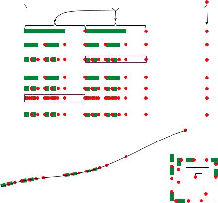
Figure 1.14 Different embeddings ξ : → R2 of code space = {0,1} in the euclidean plane lead to different metrics on . Panel (i) shows embedded in [0, 1] R at various resolutions, indicated by the numbers at the left-hand side. Zooms are shown of parts of the lines, as indicated, at resolutions 81 and 729. The red dots indicate points of ξ ( {0,1}), while the green intervals represent approximations to sets of points in ξ ( {0,1}). The two lower panels show cartoons that represent embedded in (ii) a curve and (iii) a squared spiral. One could embed in a double helix in R3 to produce an interesting metric.
that is,
|
|
|
|
|
|
m |
σn |
|
|
1 |
|
|
|
|
|
|
ξ (σ ) = n 1 |
+ |
|
|
|
||||
|
|
|
|
(N 1)n |
(N |
+ |
1)m |
|||||
|
= |
|
· · · |
|
|
= |
+ |
|
|
|
|
|
for all σ |
|
|
A |
|
|
|
|
|
|
|||
|
σ1σ2σ3 |
|
σm |
|
. See Figure 1.14. It is readily verified that ξ : |
|||||||
A A → [0, 1] |
is |
one-to-one |
and consequently |
that ( A A, d|A|) is a |
||||||||
metric space, where |
|
|
|
|
|
|
|
|
|
|||
d|A|(σ, ω) = |ξ (σ ) − ξ (ω)| = deuclidean(ξ (σ ), ξ (ω)) |
for all σ, ω A A. |
|||||||||||
We now summarize what we have proved: |
|
|
|
|||||||||
T h e o r e m 1.6.4 |
Both |
( A A, d ) and |
( A A, d|A|) are metric |
|||||||||
spaces.

32 |
Codes, metrics and topologies |
Figure 1.15 The code space {0,1} {0,1} has here been embedded in a tree-like structure in R2.
E x e r c i s e 1.6.5 Compute d (σ, ω) and d|A|(σ, ω), where σ = 010 and
|
|
|
|
|
|
|
|
|
|
|
|
|
|
ω = 0010101010 · · · = 0010. |
|
|
|
|
|||||||
E x e r c i s e 1.6.6 |
Show that ( A, d ) is a metric space, where |
|
||||||||||
d |
(σ, ω) : |
∞ |
|
σn |
ωn | |
for all σ, ω |
|
|
|
. |
||
n 1 |
(| |
|
− 1)n |
|
A |
|||||||
|
= |
|
|
|
|
|
|
|||||
|
|
= |
|A| + |
|
|
|
|
|
|
|
||
Show that d|A| and d are equivalent metrics.
E x e r c i s e 1.6.7 Show that ( A, d|A|) and ( A, d ) are not equivalent. Explain ‘geometrically’ why this is so. Hint: Think how you might try to embed A in say R2 in such a way that the euclidean metric induces the metric d on A.
E x e r c i s e 1.6.8 Here we describe an embedding of {0,1} {0,1} in R2 that looks like all the nodes, {0,1}, of a ‘tree’ together with the tips of all of the ‘twigs’,{0,1}, of the tree, as illustrated in Figure 1.15. This figure shows the relationship
between |
|
and |
0,1 |
} |
. We define ξ : 0,1 |
} |
|
|
|
→ |
R2 |
simply by |
||||||||||||||||||||
|
{0,1} |
|
|
|
|
{ |
|
|
|
|
|
|
1 |
m |
|
{ |
|
|
A |
|
|
|
|
5 |
|
m , |
||||||
|
ξ (σ1 |
σ2 |
|
|
σm ) |
|
σk |
|
|
0.499 |
|
|
, 1 |
|
|
|
|
|||||||||||||||
|
|
|
|
|
|
|
|
|
|
|
|
|
|
|
|
|
||||||||||||||||
|
· · · |
= |
2 |
k 1 |
2 |
+ |
|
− |
8 |
|||||||||||||||||||||||
|
|
|
|
|
|
|
|
|
|
|
|
|
|
|
|
|||||||||||||||||
|
|
|
|
|
|
|
|
|
|
|
|
|
|
|
|
= |
|
|
|
|
|
|
|
∞ |
|
|
|
|
|
0.499 , 1 . |
||
ξ ( ) |
|
|
|
1 |
|
, 0 |
|
|
and |
ξ (σ1σ2σ3 |
|
|
) |
1 |
|
|
σk |
|
|
|
||||||||||||
|
|
|
|
|
|
|
|
|
|
|
|
|
|
|
|
|
||||||||||||||||
= |
2 |
|
|
· · · |
2 |
k 1 |
2 |
|
+ |
|||||||||||||||||||||||
|
|
|
|
|
|
|
|
|
|
|
|
|
= |
|
|
|
|
|||||||||||||||
|
|
|
|
|
|
|
|
|
|
|
|
|
|
|
|
|
|
|
|
|
|
|
|
|
= |
|
|
|
|
|
|
|
Verify that ξ is one-to-one and write down the corresponding metric on {0,1}{0,1}. Is this new metric equivalent to d2?
Later on we will introduce other metric spaces. Given a mathematical set-up it is often worth looking for associated metric spaces, since then one has not
1.7 Cauchy sequences, limits and continuity |
33 |
only a more geometrical way of looking at the set-up but also the possibility of using contraction mapping methods, as will be discussed in Chapter 2. Contraction mapping methods are used in a number of different settings in this book to prove the existence of various types of fractal.
1.7Cauchy sequences, limits and continuity
In this section we define Cauchy sequences, limits, completeness and continuity. These important concepts are related in particular to the construction and existence of various types of fractal object. We also note some ways in which these concepts relate to code spaces.
D e f i n i t i o n 1.7.1 Let (X, d) be a metric space. Then a sequence of points {xn }∞n=1 X is said to be a Cauchy sequence iff given any > 0 there is a positive integer N > 0 such that
d(xn , xm ) < whenever n, m > N .
The sequence {xn }∞n=1 X is said to converge (in the metric d) to a point x X iff given any > 0 there is a positive integer N > 0 such that
|
d(xn , x) < |
whenever n > N . |
|||||||||||
In this case x is called the limit of {xn }n∞=1, and we write |
|||||||||||||
|
|
|
|
nlim |
xn = x. |
|
|
|
|||||
|
|
|
|
|
→∞ |
|
|
|
|
|
|
|
|
E x e r c i s e 1.7.2 |
Show that the sequence of points {xn = 1/n : n = 1, 2, . . . } |
||||||||||||
R converges to the point x = 0 in the euclidean metric. |
|
||||||||||||
E x e r c i s e 1.7.3 |
Show that the sequence of points |
|
|
||||||||||
|
σ |
AB AB |
|
|
|
|
∞ |
|
|
|
|||
|
· · · |
AB AB |
|
|
{ A,B} |
||||||||
|
n = |
|
|
|
|
|
|
|
|
||||
|
|
|
n |
|
|
|
|
n=1 |
|
|
|
||
|
|
|
|
times |
|
|
|
|
|
|
|
||
is a Cauchy sequence in each of the metric spaces d and d|A|.
It is easy to see by using the triangle inequality, d(xn , xm ) ≤ d(xn , x) + d(xm , x), that if {xn }∞n=1 converges to x then {xn }∞n=1 is a Cauchy sequence. But the converse is not true. For example, {xn = 1/n : n = 1, 2, . . . } is a Cauchy sequence in the metric space ((0, 1), deuclidean) but it has no limit in the space. So we make the following definition:
D e f i n i t i o n 1.7.4 A metric space (X, d) is said to be complete iff whenever {xn }∞n=1 X is a Cauchy sequence it converges to a point x X. We say that a subset S X is complete if the space (S, d) is complete.
34 |
Codes, metrics and topologies |
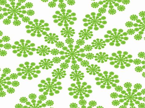
Figure 1.16 A subspace of R2 is represented in green. It consists of a centrally symmetrical pattern of ‘snowflakes’ that converge, along radial paths, towards the central point. But imagine that the point at the centre is missing, that it is not part of the subspace. Then the subspace is incomplete. Each snowflake is made of smaller snowflakes. Imagine that the centres of all the snowflakes are missing, regardless of the sizes, however small. Then, does any Cauchy sequence of points in the subspace have a limit point in the subspace?
The spaces (Rn , deuclidean) for n = 1, 2, 3, . . . are complete. So are ([0, 1], deuclidean) and ( , deuclidean). But the spaces ((0, 1), deuclidean) and (B := {(x, y) R2 : x2 + y2 < 1}, deuclidean) are not complete. Figure 1.16 illustrates an incomplete metric space.
A useful example of a complete metric space is (C[a, b], dmax), where C[a, b] denotes the set of all continuous functions f : [a, b] → R, −∞ < a < b < +∞, and
dmax( f, g) = max{| f (x) − g(x)| : x [a, b]}.
This maximum is a finite real number, as you will remember from elementary calculus. The fact that (C[a, b], dmax) is complete provides a simple demonstration of the existence of certain fractal interpolation functions.
T h e o r e m 1.7.5 Let d be either d or d|A|. Then the metric spaces ( AA, d) and ( A, d) are complete. But the metric space ( A, d) is not complete.

1.7 Cauchy sequences, limits and continuity |
35 |
The closure, defined in Section 1.8, of A in ( A A, d) is A A, that is,
A = A A.
P r o o f We prove that ( A, d) is complete where d is either d or d|A|. Let N be given. Then, in both cases, we can choose δ > 0 so small that σ, ω A must agree through the first N terms of their expansions whenever d(σ, ω) < δ.
Now let {σn }n∞=1 A. Then we can |
find an integer M(N ) such that |
d(σn , σm ) < δ whenever n, m ≥ M(N ), and consequently |
|
σn,k = σm,k for k = 1, 2, . . . , N |
whenever n, m ≥ M(N ), |
where we write |
|
σn = σn,1σn,2σn,3 · · · .
Now let
σ = σM(1),1σM(2),2σM(3),3 · · · .
Then σn agrees with σ through the first N terms whenever n ≥ M(N ).
Now let > 0 be given. Then we can choose N such that d(σ, ω) < whenever σ and ω agree through the first N terms. It follows that d(σ, σn ) < whenever n ≥ M(N ), from which it follows that limn→∞ σn = σ .
To establish that ( A A, d) is complete we simply note that the above argument applies equally well in the more general setting if we adopt the following conventions. (i) We say that the expansions of σ A and ω A agree through K terms iff either (a) K is less than or equal to both |σ | and |ω| and σn = ωn for n = 1, 2, . . . , K or (b) σ = ω. (ii) We say that the expansions of σ A and
ωA agree through K terms iff σn = ωn for n = 1, 2, . . . , min{|σ | , K }. Finally, A is not complete since the alphabet A contains at least one symbol
A, and A does not contain the limit of the Cauchy sequence
∞
σ |
n = |
A A A |
· · · |
A |
|
. |
||||
|
|
|
|
|
|
A |
||||
|
|
|
|
|
|
|
|
|
||
n times |
n=1 |
|
|
We omit the proof of the last assertion in the theorem.
D e f i n i t i o n 1.7.6 Let (X, dX ) and (Y, dY ) be metric spaces. Then a function
f : (X, dX ) → (Y, dY )
is said to be continuous at a point x iff, given any > 0, there is a δ > 0 (which may vary depending on x and ) such that
dY ( f (x), f (y)) < whenever dX (x, y) < δ with x, y X;

36 |
Codes, metrics and topologies |
f : X → Y is said to be continuous iff it is continuous at every point x X, and it is said to be uniformly continuous iff moreover it is possible to choose δ so that it does not depend on x.
A transformation from a metric space into itself can be thought of as picking up a duplicate copy of the space, deforming it, breaking it up, perhaps, and putting it back into the original space, so that each point of the space may be moved to a new point. A continuous transformation is one that does not tear or rip the space, in the sense that nearby points are carried to nearby points. But it can stretch and squeeze it hugely. For example the transformation f : (0, ∞) → (0, ∞) defined by f (x) = 1/x is continuous.
It is easy to see that if f : X → Y is continuous then it is continuous on any subset S X, that is, f |S : S X → Y is continuous.
T h e o r e m 1.7.7 The embedding mapping ξ : ( A A, d) → ([0, 1], deuclidean) is continuous where d is either d or d|A|.
P r o o f First consider the case of the mapping ξ : ( A, d ) → [0, 1]. We have
deuclidean(ξ (σ ), ξ (ω)) = |ξ (σ ) − ξ (ω)|
= |
∞ |
σn |
− |
ωn |
≤ |
∞ |
N |
|
1 |
|
|
n 1 |
(N |
1)n |
|
|
= |
|
|
, |
|||
|
m 1 (N 1)n |
(N 1)m |
|||||||||
|
|
+ |
|
n |
|
+ |
|
+ |
|
||
= |
|
|
|
= + |
|
|
|||||
|
|
|
|
|
|
|
|
|
|
|
|
where m is the number of initial successive agreements between σ and ω. The right-hand side here is smaller than > 0 for all m > M, when M is chosen to be sufficiently large. But by choosing d (σ, ω) smaller than δ = 1/2M we ensure that m is larger than M.
Similarly, consider the mapping ξ : ( A, d ) → [0, 1] and let σ, ω A. Without loss of generality we assume that |σ | ≤ |ω|. Then, much as above, we find that
max{|σ |,|ω|} |
|
N |
|
|
|
1 |
|
|
||
n |
|
|
|
|
|
|
|
|
|
|
deuclidean(ξ (σ ), ξ (ω)) = |ξ (σ ) − ξ (ω)| ≤ |
+ |
1 |
(N |
+ |
1)n |
< |
(N |
+ |
1)m |
, |
= |
|
|
|
|
|
|
||||
m |
|
|
|
|
|
|
|
|
|
|
where m is the number of initial successive agreements between σ and ω, and the value of δ > 0 is the same for a given > 0.
Finally we consider the case ξ : ( A A, d|A|) → [0, 1]. But now
deuclidean(ξ (σ ), ξ (ω)) = d|A|(σ, ω),
so whenever the right-hand side is smaller than δ = the left-hand side is too!
E x e r c i s e 1.7.8 Imagine a transformation f : R2 → R2 of the following type: all the points in are transferred to a magical (infinitely thin) sheet of paper,
1.8 Topological spaces |
37 |
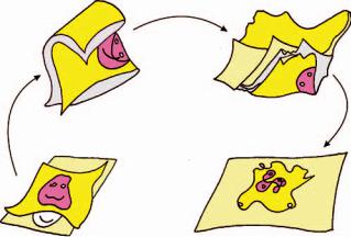
Figure 1.17 Picture of a ‘clingfilm’ transformation.
which is then picked up, folded, crumpled and squashed perfectly flat back onto R2, thus defining the transformed locations of the original points. Argue that f is continuous but that if the paper was ripped in the process then f would not be continuous. What happens if, in addition to being crumpled, the paper is stretched, this way and that, with no ripping? See Figure 1.17.
E x e r c i s e 1.7.9 Let X be the space of continuous functions |
f : [0, 1] → R |
|||||||||
and let d( f, g) := max{| f (x) − g(x)| : x [0, 1]} for all f, g X. Show |
that |
|||||||||
(X, d) is a metric space. |
|
|
|
|
|
|
|
|
|
|
E x e r c i s e 1.7.10 |
Let |
= |
|
A |
, and let α |
A |
. Define wα : |
→ |
by |
|
wα (σ ) = ασ for all |
|
|
A |
|
|
|
||||
σ . |
Show |
that wα is continuous with |
respect to the |
|||||||
metric d .
1.8 Topological spaces
In this section we introduce a third type of property that a space may possess, namely, a topology.
A topology provides a wonderful method and language for organizing the points of a space by studying and describing properties of the space that are somehow geometrical but to which most of the ‘standard’ geometrical concepts do not apply. The space is considered to be more like a jelly, even protoplasmic, rather than rigid. There is no sense of length, angle, fractal dimension, area and so on. What is under consideration is the concept of how points are related to other points by virtue of the kinds of subset of the space to which they belong. In particular, topology is the study of properties of mathematical objects that are preserved by a general class of transformations called homeomorphisms. Later we will become more and more geometrical, studying properties of sets that are preserved by more

38 |
Codes, metrics and topologies |
restrictive classes of transformations – many of which are homeomorphisms – such as euclidean transformations, affine transformations or projective transformations.
Topological concepts are absolutely essential as part of our language for describing fractals.
D e f i n i t i o n 1.8.1 |
A topological space (X, T) is a space X together with |
||||||||||
a topology T = T(X). A topology T for X is a set of subsets of X such that |
|
|
|||||||||
(i) , X T, |
|
|
|
|
|
|
|
|
|
||
(ii) if {Oi |
: i I} T is any collection of members of T then |
i INOi T, |
|
||||||||
{ |
: n |
= |
1, 2, . . . , N |
} |
is any finite set of members of T then |
n=1 |
O |
|
|
T. |
|
(iii) if On |
|
|
|
|
|
|
|
|
n |
|
|
When it is clear from the context what the topology is, or the particular topology does not matter, we sometimes write X in place of (X, T).
The sets of T are called open sets.
Any set C X that can be written, for some O T, in the form
C = X\O := {x X : x / O}
(which reads: C equals the set of elements of X that are not in O) is called a closed set.
Let O T and let x O; then O is called a neighbourhood of x. The closure of a set S X is defined to be the ‘smallest’ closed set that contains S and is denoted by S, not to be confused with SSSSSS · · · . That is,
S := C.
{C S: C is closed}
A point x X is said to be an accumulation point of a set S X if every neighbourhood of x contains infinitely many points of S. Notice that an accumulation point of S may not belong to S.
E x e r c i s e 1.8.2 Show that S = S {accumulation points of S}.
A metric space (X, d) has associated with it a natural topology Td (X) in which a set O X is called open iff, for every x O, there is a real number r > 0 such that
B(x, r ) := {y X : d(y, x) < r } O.
B(x, r) is called the (open) ball of radius r centred at x. Then one readily proves that, for S X,
S := {x X : B(x, r) ∩ S = for all r > 0}.
In general, when we are dealing with a metric space and we refer to topological concepts, it will be the natural topology to which we refer. When we wish to specify the underlying metric we may write T = Td (X). So for example the metric space (X, d) is associated with the topological space (X, Td (X)).
1.8 Topological spaces |
39 |
The natural topology on any subset of Rn will always be taken to be the topology associated with the euclidean metric.
A topological space X is called a Hausdorff space when for each pair of distinct points x, y X there is always a neighbourhood of x and one of y that have no point in common.
E x e r c i s e 1.8.3 Show that if (X, d) is a metric space then (X, Td (X)) is a Hausdorff space.
E x e r c i s e 1.8.4 Let (X, d) be a metric space and let {xn }∞n=1 X converge to x, with xn = xm for all m, n = 1, 2, . . . with m =n. Show that x is an accumulation point of {xn }∞n=1 X.
Topological language allows us to generalize concepts from metric spaces to more general settings. For example:
D e f i n i t i o n 1.8.5 Let (X, T) and (Y, T ) be (topological) spaces. Then a function
f : (X, T) → (Y, T )
is said to be continuous if f −1(O) T whenever O T (i.e. if the inverse image of every open set is an open set).
One readily proves that if f : (X, d) → (Y, d ) is continuous according to Definition 1.7.6 then it is continuous according to Definition 1.8.5 (i.e. f : (X, Td (X)) → (Y, Td (Y)) is continuous.) One reason for using topological language, even in the case of metric spaces, is that it is more efficient for describing properties because it allows us to avoid ‘epsilon and delta’ language.
D e f i n i t i o n 1.8.6 A mapping f : X → Y is called open iff it carries open sets to open sets.
An example of an open mapping is any metric transformation. But the continuous function f : (R, deuclidean) → (R, deuclidean) defined by f (x) = 4x(1 − x) is not open because f ((0, 1)) = (0, 1]. In Chapter 4 we will encounter very interesting transformations on code spaces that are continuous but not open. They have applications to painting fractals in very beautiful ways.
D e f i n i t i o n 1.8.7 A mapping f : X → Y is called a homeomorphism iff it is one-to-one, onto, continuous and open.
Let f : X → Y be a homeomorphism between two spaces X and Y. Then a set O X is open iff f (O) is open, i.e. O T(X) f (O) T(Y) . That is, f is a homeomorphism iff it induces a one-to-one invertible transformation between T(X) and T(Y).