Ohrimenko+ / Barnsley. Superfractals

x

Figure 2.8 This illustrates the organization of the pixel domains w ,h in an array ( w ,h ) constituting a digital image. Here W = 4 and H = 3.

general transformations. This difficulty is related to the question: where do digital pictures come from?

Digitization

Suppose that we are given a picture P C and we wish to convert it into a digital picture PW ×H . How do we decide which colour to assign to each pixel Pw,h ?

If the picture P is assumed to belong to a class of functions which are suitably smooth or regular in some way, so that they do not vary too wildly over the domain of a pixel, then it may be easy to select a typical value of P(x) for x w,h and for each w,h ( w,h ), discretize this value and thus define Pw,h and PW ×H .

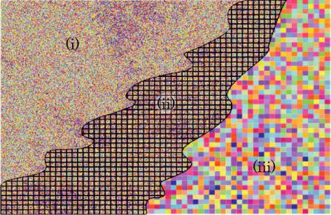
In fractal geometry, particularly, we are concerned with pictures P that may be very complicated. The problem is of the following nature: the rectangle w,h contains a vast collection of points, a countless infinity of them, each coloured in one of many possible colours, and we have to select a single representative colour for the pixel Pw,h . This idea is illustrated in Figure 2.9. Some kind of colour selection procedure is needed, perhaps based on averaging. But unless we make assumptions about the nature of the picture, for example concerning the type of function it is, thereby providing some mathematical cohesion between the colours of nearby points, then it is difficult to define a colour selection algorithm in such a way as to satisfy our intuitions about how digital pictures of different resolutions should relate to one another. We want to be able to capture the idea that we can

Figure 2.9 A mathematical picture is defined by assigning one colour to each point in a domain. How does one select the colour of a pixel to make a digital picture, an approximation to the original picture, that satisfies our intuitions? In (i) we envisage part of a mathematical picture that consists of an uncountable collection of points in the euclidean plane, each with its own colour. In (ii) part of the picture has been overlaid by a grid of domains or pixels. In (iii) each pixel has been assigned the colour of one point within it, yielding a digital picture. Vastly many different pictures many result!

increase the resolution without limit, revealing more and more intricate detail as we do so. But we do not want to prejudice the kinds of picture that we are trying to find by making assumptions about the function class they may belong to, in effect saying something about what they ‘look like’ before we have seen them.

A different model for images is provided by measure theory. This model yields a consistent way of defining digital pictures at different resolutions. Yet another type of model is provided by fractal tops, which we will encounter in Chapter 4.

2.3 Transformations of measures

At a first reading, if you do not already have some familiarity with measures, you could now read only the intuitive introduction to measures given below, study the figures in this section and then go straight on to Section 2.4. Try not to get bogged down at this point.

Intuitive description of some measures

Firstly we present an intuitive idea of a measure on a subset R2. Then we introduce a beautiful formalism, measure theory, that captures this intuition.

of grains within a subset S may provide a total amount of brightness of the red, green and blue components of light emitted by S, yielding ν(S). But S needs to be a subset of of a special type, called ‘measurable’.

Let us suppose two things. First, that we have a certain magical luminous powder. This powder glows. It has the total brightness of one candle. But it is also infinitely fine, so that its individual particles emit no light. Second, suppose that the luminous powder can be attached to the points of the euclidean plane.

All the powder could be attached to a single point x0 R2. Then x0 would glow with the brightness of one candle. Or all the powder could be attached uniformly to a line segment L . Then the line segment would glow with the brightness of one candle. But if we were to look more and more closely at one part of the line then the brightness of the observed part would steadily diminish towards zero. Or again, the powder could be distributed on unevenly, some of it concentrated on the forms of clouds and some of it filling in the shape of the moon, say, to produce a picture of varying brightness but emitting in total the light of one candle.

Similarly we may model arbitrary coloured images in this intuitive manner. We have illustrated this idea in Figure 2.10.

However, we cannot describe a measure by means of a picture function P :R2 → C. For example, if all the luminous powder were concentrated on a single point x0 then we would have to take P(x) = 0 for all x with x =x0. Digitized versions of such a picture function would tend to take the value zero everywhere. A similar problem would occur if the powder were attached uniformly to the points of a line segment L .

Figure 2.11 A measure with red, green and blue components has here been digitized to produce digital pictures with two different resolutions. The digital picture on the left has one quarter the resolution of that on the right. In principle, with uniform lighting both pictures should reflect the same number of red, green and blue photons per second, from each little pixel domain corresponding to the lower-resolution image. In practice, printing and saturation effects make this only an approximate statement. Nonetheless, try moving back from the two pictures until you cannot tell them apart.

You may at this point be tempted to try to describe the distribution of luminous powder generally with the aid of picture functions that involve ‘densities’ and ‘delta functions’. But this is not generally possible either: to see why, imagine that all the powder were attached to a non-denumerable totally disconnected subset of , or to the set of points in whose coordinates are pairs of numbers having binary expansions that contain more zeros than ones asymptotically. Neither of these methods by which powder is attached to points in R2 can be described in the usual way by densities or delta functions.

However, given any distribution of the luminous powder on , we can in fact imagine how it may be used to deduce a corresponding digital picture in a consistent manner. To each pixel Pw,h we simply assign a value equal to the total brightness of the powder lying upon the rectangle w,h , some number such as 0.01 candlepower. In this way, if a single pixel is treated as being made of smaller pixels, the sum of the brightness of the smaller pixels is equal to the brightness of the larger one, component by component.

In Figure 2.11 we show two digital pictures, one at one quarter the resolution of the other, both with the same domain R2 corresponding to the same measure. Limitlessly, new detail in the image is revealed as the resolution is increased, because the underlying measure is a fractal one, as we shall understand better in Chapter 5. See also Figure 2.12.

A σ -algebra may also be called a σ -field. The focus of our interest is on σ - algebras but it is convenient to work with fields and then extend the results to the corresponding σ -algebras. For example, the pixel field described in Exercise 2.3.5 below does not contain rectangles whose dimensions are irrational numbers, yet we are certainly going to want to discuss the ‘mass’ contained in such rectangles.

Given any space X one can always find at least one σ -algebra on X, namely S(X), the space of all subsets of X. Indeed, S(X) is the largest σ -algebra on X since it contains all other σ -algebras on X. The pair of sets {X, } is also a σ -algebra on X, as is the set of sets {X, S, X\S, } where S X.

One way to construct a σ -algebra is as follows. Start with any collection G of subsets of X. Let F (X) be the set of all sets that can be described by finite-length expressions (that make sense) involving the space X together with the sets of G,

using unions and complements. So if G1, G2 G then examples of members of F (X) are:

G1, G2, G1 G2, (X\G1) G2, ((X\G2) G2) ∩ G1, . . .

You can verify that F (X) is a field by checking that if the sets O, O1, O2 X are defined by such expressions then so are the expressions in Definition 2.3.1(i), (ii). We call F (X) the field generated by G.

E x e r c i s e 2.3.2 Prove that you generate exactly the same set F (X) if you allow intersections, as well as unions and complements, in the above description.

Let FG (X) denote the intersection of all the σ -algebras on X that contain G. Then it is straightforward to verify that FG (X) is also a σ -algebra. It is called the

σ -algebra generated by G.

E x e r c i s e 2.3.3 Prove that FG (X) is a σ -algebra.

It is convenient to think of FG (X) as the smallest σ -algebra on X that contains the field F (X).

Gpixels = w,W,hH : w = 1, 2, . . . , W ; h = 1, 2, . . . , H ; W N; H N

denote the set of all domains of all pixels of all digital images with domain R2 and having lower left corner (0, 0) and upper right corner (1, 1). Then let us call

F ( ) the pixel field for R2. Similarly, let us call FGpixels ( ) the pixel σ - algebra for R2. Show that the area of each element of F ( ) is a rational

Figure 2.13 This represents the sets in a σ -algebra FG ( ) of subsets of R2. It is generated by a pair of sets G, top left, each of which looks like the silhouette of a flower.

number. Show that S FGpixels ( ), where

√

S = (x, y) : 0 < x, y < 4 2 .

√

Show that the area of S is 2. Conclude that S is not in the pixel field but that it is in the pixel σ -algebra.

E x e r c i s e 2.3.6 Recall that a cylinder set of the code space A is a set that can be written in the form

C(σ ) := {ω A : ωn = σn for all n = 1, 2, . . . , |σ |},

for some σ A. Let F ( A) and F( A) denote respectively the field and the σ - algebra generated by the cylinder subsets of A. Let A = {0, 1}. Show that the set

S := {σ A : σn = 1 when n is an odd integer}

is in F( A) but not in F ( A).

An important σ -algebra for digital pictures is that generated by the open subsets of R2, because it is preserved by continuous transformations.

D e f i n i t i o n 2.3.7 Let (X, T(X)) be a topological space. Then the set of Borel subsets of X is the σ -algebra FT(X)(X) generated by the open subsets T(X) of X. We denote the Borel subsets of X by B(X), namely

B(X) := FT(X)(X).

E x e r c i s e 2.3.8 Show that the pixel σ -algebra for R2 is the same as the set of the Borel subsets of B( ), where the underlying topology is the natural topology induced by the euclidean metric. That is,

B( ) = FGpixels ( ).

See also Exercise 1.9.5.

Definition of a measure

D e f i n i t i o n 2.3.9 A measure on a space X is a function ν : F(X) → [0, ∞), where F(X) is a field, with

∞ ∞

On ∩ Om =

for all n, m N with n =m. In other texts a measure as defined here may be called a finite measure. Sometimes, too, it may be referred to as a positive measure.

When ν(X) = 1 the measure ν may be called a normalized measure or a probability measure on X. When F(X) = B(X), the Borel σ -algebra, the measure ν may be called a Borel measure. We denote the set of Borel measures on X by M(X) and the set of normalized Borel measures on X by P(X).

Let (X, d) be a metric space and let μ be a Borel measure. Then the support of μ is the set of points x X such that μ(Ox ) > 0 whenever Ox is an open set that contains x.

Examples of measures

E x a m p l e 2.3.10 Suppose that X consists of an array of 50 × 70 points and that Figure 2.13 represents a σ -algebra F(X). (That is, suppose that each panel in Figure 2.13 represents an array of 50 × 70 dots, some black and the others white and that the black dots within the panel represent the members of X in the corresponding subset.) Then define ν(B) to be the number of black dots in the set B, for each B F(X). Then ν : F(X) → {0, 1, . . . , 3500} is an example of a measure. In this case ν(X) = 3500.

E x e r c i s e 2.3.11 Assign a value ν(B) {0, 1, . . . , 3500} to each of the panels B in Figure 2.13 so as to define a measure on the σ -algebra F(X) in Example 2.3.10.

subsets of the code space A, as in Exercise 2.3.6. Let A = {1, 2, . . . , N }. Let p1 ≥ 0, p2 ≥ 0, . . . , pN ≥ 0 and p0 + p1 + · · · + pN = 1. Then there is a unique measure ν on the field F ( A) generated by the cylinder subsets {C(σ ) : σ } such that

ν (C(σ )) = pσ1 pσ2 · · · pσ|σ | for all σ .

Let us say that the length of the cylinder subset C(σ ) is |σ |. Then it is straightforward to show that any element of F ( A) may be written as a union of cylinder subsets of the same length, and also that distinct cylinder subsets of the same length are disjoint. It follows that the measure of any element of the field F ( A) can be written as the sum of numbers of the form pσ1 pσ2 · · · pσ|σ | for some fixed value of |σ |.

E x a m p l e 2.3.14 Let ρ : R2 → [0, ∞) be a continuous positive function. It describes a surface over . Using standard integration, one can in principle evaluate the integral

ν ( w,h ) := w,h ρ(x, y)dxdy.

This yields the volume between the part of the surface lying ‘vertically above’ the rectangle w,h and the x y-plane. In a similar manner one can evaluate ν (S) for any set S in the pixel field F ( ). Then it can be shown (straightforwardly) that ν : F ( ) → [0, ∞) is a measure. In this case the measure is indeed described by the density function ρ(x, y). This same construction of a measure works equally well if the density function is piecewise continuous and its discontinuities occur on sets that are not too complicated, for example boundaries of domains of pixels.

Digital pictures of measures

Given any vector of measures,

νρ = (ν1, ν2, ν3),

where νi is a measure on the pixel field F ( ) for i = 1, 2, 3, we can uniquely specify a corresponding digital picture PW ×H for each W, H N. The members of the resulting family of digital pictures will be consistent with one another in this sense: the value of any pixel Pw,h will be greater than or equal to the sum of the values of any set of pixels from a family whose domains are disjoint and whose union is contained in w,h , while Pw,h will be less than or equal to the sum of the values of any set of pixels from a family whose union contains w,h .

However, in order to be able to discuss what happens when we transform a measure, say under a continuous transformation, we need to know the value of the measure not just on the pixel field but also on the pixel σ -algebra, because pixels are not transformed into pixels by general transformations. Luckily, the following theorem tells us two wonderful things, that once we have a measure on a field we can extend it uniquely to the σ -algebra generated by the field and also how to evaluate the measure on the σ -algebra using only its values on the field.

T h e o r e m 2.3.15 Let X be a space, let F (X) be a field on X and let F(X) be the smallest σ -algebra on X that contains F (X). Let ν : F (X) → [0, ∞) be a measure. Then there exists a unique measure ν : F(X) → [0, ∞) such that

for all A F(X).

The notation inf S, where S R {−∞, +∞}, means the largest number in R {−∞, +∞} that is less than or equal to all the numbers in the set S. For example, inf R = −∞, inf(1, 2] = 1 and inf{1/n : n = 1, 2, . . . } = 0. Similarly