Analytic center of linear matrix inequality
minimize |
− log det X |
subject to |
tr(AiX) = bi, i = 1, . . . , p |
variable X Sn
optimality conditions
Xp
X 0, −(X )−1 + νj Ai = 0, tr(AiX ) = bi, i = 1, . . . , p
j=1
Newton equation at feasible X:
Xp
X−1 XX−1 + wjAi = X−1, tr(Ai X) = 0, i = 1, . . . , p
j=1
• follows from linear approximation (X + X)−1 ≈ X−1 − X−1 XX−1
• n(n + 1)/2 + p variables X, w
Equality constrained minimization |
11–18 |
solution by block elimination
|
eliminate X from first equation: |
p |
|
• |
X = X − Pj=1 wjXAjX |
|
substitute X in second equation |
|
• |
|
|
|
|
p |
|
|
|
X |
|
|
|
tr(AiXAjX)wj = bi, i = 1, . . . , p |
(2) |
j=1
a dense positive definite set of linear equations with variable w Rp
flop count (dominant terms) using Cholesky factorization X = LLT :
•form p products LT AjL: (3/2)pn3
•form p(p + 1)/2 inner products tr((LT AiL)(LT AjL)): (1/2)p2n2
•solve (2) via Cholesky factorization: (1/3)p3
Equality constrained minimization |
11–19 |
Convex Optimization — Boyd & Vandenberghe
12.Interior-point methods
•inequality constrained minimization
•logarithmic barrier function and central path
•barrier method
•feasibility and phase I methods
•complexity analysis via self-concordance
•generalized inequalities
Inequality constrained minimization
minimize |
f0(x) |
|
subject to |
fi(x) ≤ 0, i = 1, . . . , m |
(1) |
|
Ax = b |
|
•fi convex, twice continuously di erentiable
•A Rp×n with rank A = p
•we assume p is finite and attained
•we assume problem is strictly feasible: there exists x˜ with
x˜ dom f0, fi(˜x) < 0, i = 1, . . . , m, Ax˜ = b
hence, strong duality holds and dual optimum is attained
Interior-point methods |
12–2 |
Examples
•LP, QP, QCQP, GP
•entropy maximization with linear inequality constraints
minimize |
|
n |
|
|
|
i=1 xi log xi |
subject to |
F x |
|
g |
P |
|
|
Ax = b
with dom f0 = Rn++
•di erentiability may require reformulating the problem, E.G., piecewise-linear minimization or ℓ∞-norm approximation via LP
•SDPs and SOCPs are better handled as problems with generalized inequalities (see later)
Interior-point methods |
12–3 |
Logarithmic barrier
reformulation of (1) via indicator function:
minimize |
f0(x) + |
m |
I |
|
(f |
(x)) |
subject to |
Ax = b |
Pi=1 |
|
− |
i |
|
where I−(u) = 0 if u ≤ 0, I−(u) = ∞ otherwise (indicator function of R−)
approximation via logarithmic barrier
minimize |
f0(x) − (1/t) |
P |
m |
− |
fi(x)) |
i=1 log( |
subject to |
Ax = b |
|
|
•an equality constrained problem
•for t > 0, −(1/t) log(−u) is a smooth approximation of I−
•approximation improves as t → ∞
Interior-point methods |
12–4 |
logarithmic barrier function
Xm
φ(x) = − log(−fi(x)), dom φ = {x | f1(x) < 0, . . . , fm(x) < 0}
i=1
•convex (follows from composition rules)
•twice continuously di erentiable, with derivatives
|
m |
|
|
|
|
φ(x) = |
X − |
1 |
|
fi(x) |
|
|
|
|
|
|
i=1 |
|
fi(x) |
|
|
|
|
|
|
m |
|
|
|
|
2φ(x) = |
X |
|
1 |
fi(x) fi(x)T |
|
|
|
|
i=1 |
fi(x)2 |
|
|
|
|
|
|
m |
|
|
+ |
X − |
1 |
2fi(x) |
|
|
|
|
|
i=1 |
fi(x) |
|
|
|
Interior-point methods |
12–5 |
Central path
• for t > 0, define x (t) as the solution of
minimize |
tf0(x) + φ(x) |
subject to |
Ax = b |
(for now, assume x (t) exists and is unique for each t > 0)
• central path is {x (t) | t > 0}
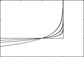
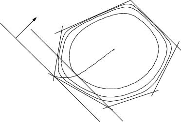
example: central path for an LP
minimize |
cT x |
subject to |
aiT x ≤ bi, i = 1, . . . , 6 |
hyperplane cT x = cT x (t) is tangent to level curve of φ through x (t)
c
x 
 x (10)
Interior-point methods |
12–6 |
Dual points on central path
x = x (t) if there exists a w such that
|
m |
|
|
t f0(x) + |
X − |
1 |
fi(x) + AT w = 0, Ax = b |
|
|
|
|
|
i=1 |
fi(x) |
|
|
|
• therefore, x (t) minimizes the Lagrangian
Xm
L(x, λ (t), ν (t)) = f0(x) + λi (t)fi(x) + ν (t)T (Ax − b)
i=1
where we define λi (t) = 1/(−tfi(x (t)) and ν (t) = w/t
• this confirms the intuitive idea that f0(x (t)) → p if t → ∞:
p ≥ g(λ (t), ν (t))
=L(x (t), λ (t), ν (t))
=f0(x (t)) − m/t
Interior-point methods |
12–7 |
Interpretation via KKT conditions
x = x (t), λ = λ (t), ν = ν (t) satisfy
1.primal constraints: fi(x) ≤ 0, i = 1, . . . , m, Ax = b
2.dual constraints: λ 0
3.approximate complementary slackness: −λifi(x) = 1/t, i = 1, . . . , m
4.gradient of Lagrangian with respect to x vanishes:
Xm
f0(x) + λi fi(x) + AT ν = 0
i=1
di erence with KKT is that condition 3 replaces λifi(x) = 0
Interior-point methods |
12–8 |