

[Boyd]_cvxslides
.pdfGeometric interpretation
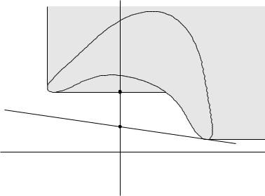
for simplicity, consider problem with one constraint f1(x) ≤ 0 interpretation of dual function:
g(λ) = |
inf |
(t + λu), |
where |
|
(u,t)G |
|
|
|
|
t |
|
|
|
G |
|
|
|
p |
|
λu + t = g(λ) |
|
g(λ) |
|
|
|
|
|
|
|
|
u |
G = {(f1(x), f0(x)) | x D} |
t |
G |
p |
d |
u |
•λu + t = g(λ) is (non-vertical) supporting hyperplane to G
•hyperplane intersects t-axis at t = g(λ)
Duality |
5–15 |
epigraph variation: same interpretation if G is replaced with
A = {(u, t) | f1(x) ≤ u, f0(x) ≤ t for some x D} |
|
|
t |
|
A |
λu + t = g(λ) |
p |
|
|
|
g(λ) |
|
u |
strong duality
•holds if there is a non-vertical supporting hyperplane to A at (0, p )
•for convex problem, A is convex, hence has supp. hyperplane at (0, p )
•Slater’s condition: if there exist (˜u, t˜) A with u˜ < 0, then supporting hyperplanes at (0, p ) must be non-vertical
Duality |
5–16 |
Complementary slackness
assume strong duality holds, x is primal optimal, (λ , ν ) is dual optimal
f0(x ) = g(λ , ν ) = |
x |
f0(x) + |
i fi(x) + |
i hi |
! |
||
|
|
|
|
m |
|
p |
|
|
|
|
|
X |
|
X |
|
|
|
|
inf |
|
λ |
ν |
(x) |
|
|
|
|
i=1 |
|
i=1 |
|
|
|
|
|
m |
p |
|
|
|
|
|
|
X |
X |
|
|
|
|
≤ f0(x ) + λi fi(x ) + |
νi hi(x ) |
||||
|
|
|
|
i=1 |
i=1 |
|
|
|
|
≤ |
f0(x ) |
|
|
|
|
hence, the two inequalities hold with equality
•x minimizes L(x, λ , ν )
•λi fi(x ) = 0 for i = 1, . . . , m (known as complementary slackness):
λi > 0 = fi(x ) = 0, fi(x ) < 0 = λi = 0
Duality |
5–17 |
Karush-Kuhn-Tucker (KKT) conditions
the following four conditions are called KKT conditions (for a problem with di erentiable fi, hi):
1.primal constraints: fi(x) ≤ 0, i = 1, . . . , m, hi(x) = 0, i = 1, . . . , p
2.dual constraints: λ 0
3.complementary slackness: λifi(x) = 0, i = 1, . . . , m
4.gradient of Lagrangian with respect to x vanishes:
m |
p |
X |
X |
f0(x) + |
λi fi(x) + νi hi(x) = 0 |
i=1 |
i=1 |
from page 5–17: if strong duality holds and x, λ, ν are optimal, then they must satisfy the KKT conditions
Duality |
5–18 |
KKT conditions for convex problem
|
˜ |
|
if x˜, λ, ν˜ satisfy KKT for a convex problem, then they are optimal: |
||
• |
˜ |
|
from complementary slackness: f0(˜x) = L(˜x, λ, ν˜) |
|
|
• |
˜ |
˜ |
from 4th condition (and convexity): g(λ, ν˜) = L(˜x, λ, ν˜) |
||
˜
hence, f0(˜x) = g(λ, ν˜)
if Slater’s condition is satisfied:
x is optimal if and only if there exist λ, ν that satisfy KKT conditions
•recall that Slater implies strong duality, and dual optimum is attained
•generalizes optimality condition f0(x) = 0 for unconstrained problem
Duality |
5–19 |

example: water-filling (assume αi > 0)
|
|
P |
minimize |
− |
n |
i=1 log(xi + αi) |
||
subject to |
x 0, 1T x = 1 |
|
x is optimal i x 0, 1T x = 1, and there exist λ Rn, ν R such that
λ 0, |
λixi = 0, |
1 |
|
+ λi = ν |
||||||||||||||||||
|
||||||||||||||||||||||
xi + αi |
||||||||||||||||||||||
• if ν < 1/αi: λi = 0 and xi = 1/ν − αi |
|
|
|
|
|
|
|
|
|
|
|
|
|
|
|
|
|
|
|
|
|
|
• if ν ≥ 1/αi: λi = ν − 1/αi and xi = 0 |
|
|
|
|
|
|
|
|
|
|
|
|
|
|
|
|
|
|
|
|
|
|
|
n |
|
− αi} = 1 |
|||||||||||||||||||
• determine ν from 1T x = Pi=1 max{0, 1/ν |
||||||||||||||||||||||
interpretation |
|
|
|
|
|
|
|
|
|
|
|
|
|
|
|
|
|
|
|
|
|
|
• n patches; level of patch i is at height αi |
1/ν |
|
|
|
|
|
|
|
|
|
|
|
|
|
|
|
|
|
xi |
|||
|
|
|
|
|
|
|
|
|
|
|
|
|
|
|
|
|
||||||
|
|
|
|
|
|
|
|
|
|
|
|
|
|
|
|
|
||||||
|
|
|
|
|
|
|
|
|
|
|
|
|
|
|
|
|
||||||
• flood area with unit amount of water |
|
|
|
|
|
|
|
|
|
|
|
|
|
|
|
|
|
|
|
|
||
|
|
|
|
|
|
|
|
|
|
|
|
|
|
|
|
|
|
|
||||
|
|
|
|
|
|
|
|
|
|
|
|
|
|
|
|
|
|
|
||||
|
|
|
|
|
|
|
|
|
|
|
|
|
|
|
|
|
|
|
|
αi |
||
|
|
|
|
|
|
|
|
|
|
|
|
|
|
|
|
|
|
|
|
|||
|
|
|
|
|
|
|
|
|
|
|
|
|
|
|
|
|
|
|
||||
|
|
|
|
|
|
|
|
|
|
|
|
|
|
|
|
|
|
|
||||
• resulting level is 1/ν |
|
|
|
|
|
|
|
|
|
|
|
|
|
|
|
|
|
|
|
|
|
|
|
|
|
|
|
|
|
|
|
|
|
|
|
|
|
|
|
|
|
|
|
|
|
|
|
|
|
|
|
|
|
|
|
|
|
|
|
|
|
|
|
|
|
|
|
|
|
|
|
|
|
|
|
|
|
|
|
i |
|||||||||||
Duality |
5–20 |
Perturbation and sensitivity analysis
(unperturbed) optimization problem and its dual
minimize |
f0(x) |
|
maximize |
g(λ, ν) |
subject to |
fi(x) ≤ 0, |
i = 1, . . . , m |
subject to |
λ 0 |
|
hi(x) = 0, |
i = 1, . . . , p |
|
|
perturbed problem and its dual |
|
|
||
min. |
f0(x) |
|
max. |
g(λ, ν) − uT λ − vT ν |
s.t. |
fi(x) ≤ ui, |
i = 1, . . . , m |
s.t. |
λ 0 |
|
hi(x) = vi, |
i = 1, . . . , p |
|
|
•x is primal variable; u, v are parameters
•p (u, v) is optimal value as a function of u, v
•we are interested in information about p (u, v) that we can obtain from the solution of the unperturbed problem and its dual
Duality |
5–21 |
global sensitivity result
assume strong duality holds for unperturbed problem, and that λ , ν are dual optimal for unperturbed problem
apply weak duality to perturbed problem:
p (u, v) ≥ g(λ , ν ) − uT λ − vT ν = p (0, 0) − uT λ − vT ν
sensitivity interpretation
•if λi large: p increases greatly if we tighten constraint i (ui < 0)
•if λi small: p does not decrease much if we loosen constraint i (ui > 0)
•if νi large and positive: p increases greatly if we take vi < 0; if νi large and negative: p increases greatly if we take vi > 0
•if νi small and positive: p does not decrease much if we take vi > 0; if νi small and negative: p does not decrease much if we take vi < 0
Duality |
5–22 |
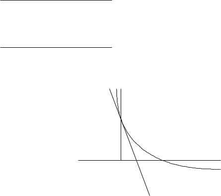
local sensitivity: if (in addition) p (u, v) is di erentiable at (0, 0), then
|
λi = − |
∂p (0, 0) |
, |
νi = − |
∂p (0, 0) |
||||
|
∂ui |
∂vi |
|
||||||
proof (for λ ): from global sensitivity result, |
|
|
|
||||||
i |
|
|
|
|
|
|
|
||
|
∂p (0, 0) |
= lim |
p (tei, 0) − p (0, 0) |
≥ − |
λ |
||||
|
|
||||||||
|
∂ui |
t 0 |
|
t |
|
i |
|||
|
∂p (0, 0) |
= lim |
p (tei, 0) − p (0, 0) |
≤ − |
λ |
||||
|
|
||||||||
|
∂ui |
t 0 |
|
t |
|
i |
|||
hence, equality
p (u) for a problem with one (inequality) |
|
constraint: |
u |
u = 0 |
p (u) |
|
p (0) − λ u |
Duality |
5–23 |
Duality and problem reformulations
•equivalent formulations of a problem can lead to very di erent duals
•reformulating the primal problem can be useful when the dual is di cult to derive, or uninteresting
common reformulations
•introduce new variables and equality constraints
•make explicit constraints implicit or vice-versa
•transform objective or constraint functions
E.G., replace f0(x) by φ(f0(x)) with φ convex, increasing
Duality |
5–24 |