

[Boyd]_cvxslides
.pdfNewton’s method with equality constraints
given starting point x dom f with Ax = b, tolerance ǫ > 0. repeat
1. Compute the Newton step and decrement xnt, λ(x).
2.Stopping criterion. quit if λ2/2 ≤ ǫ.
3.Line search. Choose step size t by backtracking line search.
4. Update. x := x + t xnt.
•a feasible descent method: x(k) feasible and f(x(k+1)) < f(x(k))
•a ne invariant
Equality constrained minimization |
11–8 |
Newton’s method and elimination
Newton’s method for reduced problem
˜
minimize f(z) = f(F z + xˆ)
• variables z Rn−p
• xˆ satisfies Axˆ = b; rank F = n − p and AF = 0
• |
˜ |
(0) |
, generates iterates z |
(k) |
Newton’s method for f, started at z |
|
|
Newton’s method with equality constraints when started at x(0) = F z(0) + xˆ, iterates are
x(k+1) = F z(k) + xˆ
hence, don’t need separate convergence analysis
Equality constrained minimization |
11–9 |
Newton step at infeasible points
2nd interpretation of page 11–6 extends to infeasible x (I.E., Ax 6= b)
linearizing optimality conditions at infeasible x (with x dom f) gives
A |
0 |
|
w |
|
− |
Ax − b |
|
2f(x) |
AT |
|
xnt |
= |
|
f(x) |
(1) |
primal-dual interpretation
• write optimality condition as r(y) = 0, where
y = (x, ν), r(y) = ( f(x) + AT ν, Ax − b)
• linearizing r(y) = 0 gives r(y + |
y) ≈ r(y) + Dr(y)Δy = 0: |
|||||
A |
0 |
|
νnt |
= − |
Ax − b |
|
2f(x) AT |
|
xnt |
|
f(x) + AT ν |
|
|
same as (1) with w = ν + |
νnt |
|
|
|
|
|
Equality constrained minimization |
11–10 |

Infeasible start Newton method
given starting point x dom f, ν, tolerance ǫ > 0, α (0, 1/2), β (0, 1).
repeat |
|
|
1. |
Compute primal and dual Newton steps |
xnt, νnt. |
2. |
Backtracking line search on krk2. |
|
|
t := 1. |
|
|
while kr(x + t xnt, ν + t νnt)k2 > (1 − αt)kr(x, ν)k2, t := βt. |
|
3. |
Update. x := x + t xnt, ν := ν + t |
νnt. |
until Ax = b and kr(x, ν)k2 ≤ ǫ. |
|
|
|
|
|
• |
not a descent method: f(x(k+1)) > f(x(k)) is possible |
• |
directional derivative of kr(y)k2 in direction y = (Δxnt, νnt) is |
dt kr(y + t y)k2 t=0 = −kr(y)k2 |
|
d |
|
|
|
|
|
Equality constrained minimization |
11–11 |
Solving KKT systems
A |
0 |
w |
= − |
h |
H |
AT |
v |
|
g |
solution methods
•LDLT factorization
•elimination (if H nonsingular)
AH−1AT w = h − AH−1g, Hv = −(g + AT w)
• elimination with singular H: write as
|
A |
0 |
w |
= − |
g + h |
|
|
H + AT QA AT |
v |
|
AT Qh |
|
|
with Q 0 for which H + AT QA 0, and apply elimination
Equality constrained minimization |
11–12 |

Equality constrained analytic centering
primal problem: minimize − |
n |
|
|
|
i=1 log xi subject to Ax = b |
||||
dual problem: maximize −b |
TP |
n |
T |
ν)i + n |
ν + Pi=1 log(A |
|
|||
three methods for an example with A R100×500, di erent starting points
1. |
Newton method with equality constraints (requires x(0) 0, Ax(0) = b) |
|||||
|
|
105 |
|
|
|
|
|
|
|
|
|
|
|
|
p |
100 |
|
|
|
|
|
) − |
|
|
|
|
|
|
|
|
|
|
|
|
|
(k) |
10−5 |
|
|
|
|
|
x |
|
|
|
|
|
|
f( |
|
|
|
|
|
|
|
10−10 |
5 |
10 |
15 |
20 |
|
|
0 |
||||
|
|
|
|
k |
|
|
Equality constrained minimization |
11–13 |
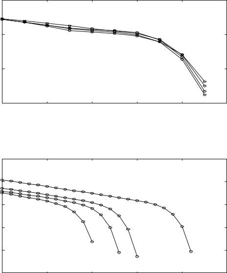
2. Newton method applied to dual problem (requires AT ν(0) 0) |
|||||||
|
|
105 |
|
|
|
|
|
|
) |
|
|
|
|
|
|
|
(k) |
100 |
|
|
|
|
|
|
− g(ν |
10−5 |
|
|
|
|
|
|
|
|
|
|
|
|
|
|
p |
|
|
|
|
|
|
|
|
10−10 |
2 |
4 |
6 |
8 |
10 |
|
|
0 |
|||||
|
|
|
|
|
k |
|
|
3. |
infeasible start Newton method (requires x(0) 0) |
|
|||||
|
|
1010 |
|
|
|
|
|
|
2 |
105 |
|
|
|
|
|
|
k |
|
|
|
|
|
|
|
) |
|
|
|
|
|
|
|
(k) |
100 |
|
|
|
|
|
|
ν |
|
|
|
|
|
|
|
, |
|
|
|
|
|
|
|
(k) |
10−5 |
|
|
|
|
|
|
kr(x |
10−10 |
|
|
|
|
|
|
|
10−15 |
5 |
10 |
15 |
20 |
25 |
|
|
0 |
|||||
|
|
|
|
|
k |
|
|
Equality constrained minimization |
11–14 |
complexity per iteration of three methods is identical
1. use block elimination to solve KKT system
|
A |
0 |
|
w |
= |
0 |
|
|
diag(x)−2 |
AT |
|
x |
|
diag(x)−11 |
|