

- •Contents
- •Symbols and Abbreviations
- •Symbols
- •Greek Symbols
- •Subscripts
- •Abbreviations
- •Preface
- •Road Map of the Book
- •The Arrangement
- •Suggested Route for the Coursework
- •First Semester
- •Second Semester
- •Suggestions for the Class
- •Use of Semi-empirical Relations
- •1 Introduction
- •1.1 Overview
- •1.1.1 What Is to Be Learned?
- •1.1.2 Coursework Content
- •1.2 Brief Historical Background
- •1.3 Current Aircraft Design Status
- •1.3.1 Forces and Drivers
- •1.3.2 Current Civil Aircraft Design Trends
- •1.3.3 Current Military Aircraft Design Trends
- •1.4 Future Trends
- •1.4.1 Civil Aircraft Design: Future Trends
- •1.4.2 Military Aircraft Design: Future Trends
- •1.5 Learning Process
- •1.6 Units and Dimensions
- •1.7 Cost Implications
- •2 Methodology to Aircraft Design, Market Survey, and Airworthiness
- •2.1 Overview
- •2.1.1 What Is to Be Learned?
- •2.1.2 Coursework Content
- •2.2 Introduction
- •2.3 Typical Design Process
- •2.3.1 Four Phases of Aircraft Design
- •2.3.2 Typical Resources Deployment
- •2.3.3 Typical Cost Frame
- •2.3.4 Typical Time Frame
- •2.4 Typical Task Breakdown in Each Phase
- •Phase 1: Conceptual Study Phase (Feasibility Study)
- •Phase 3: Detailed Design Phase (Full-Scale Product Development)
- •2.4.1 Functional Tasks during the Conceptual Study (Phase 1: Civil Aircraft)
- •2.4.2 Project Activities for Small Aircraft Design
- •Phase 1: Conceptual Design (6 Months)
- •Phase 3: Detailed Design (Product Development) (12 Months)
- •2.5 Aircraft Familiarization
- •Fuselage Group
- •Wing Group
- •Empennage Group
- •Nacelle Group
- •Undercarriage Group
- •2.6 Market Survey
- •2.7 Civil Aircraft Market
- •2.8 Military Market
- •2.9 Comparison between Civil and Military Aircraft Design Requirements
- •2.10 Airworthiness Requirements
- •2.11 Coursework Procedures
- •3 Aerodynamic Considerations
- •3.1 Overview
- •3.1.1 What Is to Be Learned?
- •3.1.2 Coursework Content
- •3.2 Introduction
- •3.3 Atmosphere
- •3.4 Fundamental Equations
- •3.5.1 Flow Past Aerofoil
- •3.6 Aircraft Motion and Forces
- •3.6.1 Motion
- •3.6.2 Forces
- •3.7 Aerofoil
- •3.7.1 Groupings of Aerofoils and Their Properties
- •NACA Four-Digit Aerofoil
- •NACA Five-Digit Aerofoil
- •NACA Six-Digit Aerofoil
- •Other Types of Aerofoils
- •3.9 Generation of Lift
- •3.10 Types of Stall
- •3.10.1 Gradual Stall
- •3.10.2 Abrupt Stall
- •3.11 Comparison of Three NACA Aerofoils
- •3.12 High-Lift Devices
- •3.13 Transonic Effects – Area Rule
- •3.14 Wing Aerodynamics
- •3.14.1 Induced Drag and Total Aircraft Drag
- •3.15 Aspect Ratio Correction of 2D Aerofoil Characteristics for 3D Finite Wing
- •3.16.1 Planform Area, SW
- •3.16.2 Wing Aspect Ratio
- •3.16.4 Wing Root (Croot) and Tip (Ctip) Chord
- •3.16.6 Wing Twist
- •3.17 Mean Aerodynamic Chord
- •3.18 Compressibility Effect: Wing Sweep
- •3.19 Wing Stall Pattern and Wing Twist
- •3.20.1 The Square-Cube Law
- •3.20.2 Aircraft Wetted Area (AW) versus Wing Planform Area (Sw)
- •3.20.3 Additional Vortex Lift
- •3.20.4 Additional Surfaces on Wing
- •3.21 Finalizing Wing Design Parameters
- •3.22 Empennage
- •3.22.1 H-Tail
- •3.22.2 V-Tail
- •3.23 Fuselage
- •3.23.2 Fuselage Length, Lfus
- •3.23.3 Fineness Ratio, FR
- •3.23.4 Fuselage Upsweep Angle
- •3.23.5 Fuselage Closure Angle
- •3.23.6 Front Fuselage Closure Length, Lf
- •3.23.7 Aft Fuselage Closure Length, La
- •3.23.8 Midfuselage Constant Cross-Section Length, Lm
- •3.23.9 Fuselage Height, H
- •3.23.10 Fuselage Width, W
- •3.23.11 Average Diameter, Dave
- •3.23.12 Cabin Height, Hcab
- •3.23.13 Cabin Width, Wcab
- •3.24 Undercarriage
- •3.25 Nacelle and Intake
- •3.26 Speed Brakes and Dive Brakes
- •4.1 Overview
- •4.1.1 What Is to Be Learned?
- •4.1.2 Coursework Content
- •4.2 Introduction
- •4.3 Aircraft Evolution
- •4.4 Civil Aircraft Mission (Payload-Range)
- •4.5 Civil Subsonic Jet Aircraft Statistics (Sizing Parameters and Regression Analysis)
- •4.5.1 Maximum Takeoff Mass versus Number of Passengers
- •4.5.2 Maximum Takeoff Mass versus Operational Empty Mass
- •4.5.3 Maximum Takeoff Mass versus Fuel Load
- •4.5.4 Maximum Takeoff Mass versus Wing Area
- •4.5.5 Maximum Takeoff Mass versus Engine Power
- •4.5.6 Empennage Area versus Wing Area
- •4.5.7 Wing Loading versus Aircraft Span
- •4.6 Civil Aircraft Component Geometries
- •4.7 Fuselage Group
- •4.7.1 Fuselage Width
- •4.7.2 Fuselage Length
- •4.7.3 Front (Nose Cone) and Aft-End Closure
- •4.7.4 Flight Crew (Flight Deck) Compartment Layout
- •4.7.5 Cabin Crew and Passenger Facilities
- •4.7.6 Seat Arrangement, Pitch, and Posture (95th Percentile) Facilities
- •4.7.7 Passenger Facilities
- •4.7.8 Cargo Container Sizes
- •4.7.9 Doors – Emergency Exits
- •4.8 Wing Group
- •4.9 Empennage Group (Civil Aircraft)
- •4.10 Nacelle Group
- •4.11 Summary of Civil Aircraft Design Choices
- •4.13 Military Aircraft Mission
- •4.14.1 Military Aircraft Maximum Take-off Mass (MTOM) versus Payload
- •4.14.2 Military MTOM versus OEM
- •4.14.3 Military MTOM versus Fuel Load Mf
- •4.14.4 MTOM versus Wing Area (Military)
- •4.14.5 MTOM versus Engine Thrust (Military)
- •4.14.6 Empennage Area versus Wing Area (Military)
- •4.14.7 Aircraft Wetted Area versus Wing Area (Military)
- •4.15 Military Aircraft Component Geometries
- •4.16 Fuselage Group (Military)
- •4.17 Wing Group (Military)
- •4.17.1 Generic Wing Planform Shapes
- •4.18 Empennage Group (Military)
- •4.19 Intake/Nacelle Group (Military)
- •4.20 Undercarriage Group
- •4.21 Miscellaneous Comments
- •4.22 Summary of Military Aircraft Design Choices
- •5 Aircraft Load
- •5.1 Overview
- •5.1.1 What Is to Be Learned?
- •5.1.2 Coursework Content
- •5.2 Introduction
- •5.2.1 Buffet
- •5.2.2 Flutter
- •5.3 Flight Maneuvers
- •5.3.1 Pitch Plane (X-Z) Maneuver (Elevator/Canard-Induced)
- •5.3.2 Roll Plane (Y-Z) Maneuver (Aileron-Induced)
- •5.3.3 Yaw Plane (Z-X) Maneuver (Rudder-Induced)
- •5.4 Aircraft Loads
- •5.4.1 On the Ground
- •5.4.2 In Flight
- •5.5.1 Load Factor, n
- •5.6 Limits – Load and Speeds
- •5.6.1 Maximum Limit of Load Factor
- •5.6.2 Speed Limits
- •5.7 V-n Diagram
- •5.7.1 Low-Speed Limit
- •5.7.2 High-Speed Limit
- •5.7.3 Extreme Points of a V-n Diagram
- •Positive Loads
- •Negative Loads
- •5.8 Gust Envelope
- •6.1 Overview
- •6.1.1 What Is to Be Learned?
- •6.1.2 Coursework Content
- •6.2 Introduction
- •Closure of the Fuselage
- •6.4 Civil Aircraft Fuselage: Typical Shaping and Layout
- •6.4.1 Narrow-Body, Single-Aisle Aircraft
- •6.4.2 Wide-Body, Double-Aisle Aircraft
- •6.4.3 Worked-Out Example: Civil Aircraft Fuselage Layout
- •6.5.1 Aerofoil Selection
- •6.5.2 Wing Design
- •Planform Shape
- •Wing Reference Area
- •Wing Sweep
- •Wing Twist
- •Wing Dihedral/Anhedral
- •6.5.3 Wing-Mounted Control-Surface Layout
- •6.5.4 Positioning of the Wing Relative to the Fuselage
- •6.6.1 Horizontal Tail
- •6.6.2 Vertical Tail
- •6.8 Undercarriage Positioning
- •6.10 Miscellaneous Considerations in Civil Aircraft
- •6.12.1 Use of Statistics in the Class of Military Trainer Aircraft
- •6.12.3 Miscellaneous Considerations – Military Design
- •6.13 Variant CAS Design
- •6.13.1 Summary of the Worked-Out Military Aircraft Preliminary Details
- •7 Undercarriage
- •7.1 Overview
- •7.1.1 What Is to Be Learned?
- •7.1.2 Coursework Content
- •7.2 Introduction
- •7.3 Types of Undercarriage
- •7.5 Undercarriage Retraction and Stowage
- •7.5.1 Stowage Space Clearances
- •7.6 Undercarriage Design Drivers and Considerations
- •7.7 Turning of an Aircraft
- •7.8 Wheels
- •7.9 Loads on Wheels and Shock Absorbers
- •7.9.1 Load on Wheels
- •7.9.2 Energy Absorbed
- •7.11 Tires
- •7.13 Undercarriage Layout Methodology
- •7.14 Worked-Out Examples
- •7.14.1 Civil Aircraft: Bizjet
- •Baseline Aircraft with 10 Passengers at a 33-Inch Pitch
- •Shrunk Aircraft (Smallest in the Family Variant) with 6 Passengers at a 33-Inch Pitch
- •7.14.2 Military Aircraft: AJT
- •7.15 Miscellaneous Considerations
- •7.16 Undercarriage and Tire Data
- •8 Aircraft Weight and Center of Gravity Estimation
- •8.1 Overview
- •8.1.1 What Is to Be Learned?
- •8.1.2 Coursework Content
- •8.2 Introduction
- •8.3 The Weight Drivers
- •8.4 Aircraft Mass (Weight) Breakdown
- •8.5 Desirable CG Position
- •8.6 Aircraft Component Groups
- •8.6.1 Civil Aircraft
- •8.6.2 Military Aircraft (Combat Category)
- •8.7 Aircraft Component Mass Estimation
- •8.8 Rapid Mass Estimation Method: Civil Aircraft
- •8.9 Graphical Method for Predicting Aircraft Component Weight: Civil Aircraft
- •8.10 Semi-empirical Equation Method (Statistical)
- •8.10.1 Fuselage Group – Civil Aircraft
- •8.10.2 Wing Group – Civil Aircraft
- •8.10.3 Empennage Group – Civil Aircraft
- •8.10.4 Nacelle Group – Civil Aircraft
- •Jet Type (Includes Pylon Mass)
- •Turboprop Type
- •Piston-Engine Nacelle
- •8.10.5 Undercarriage Group – Civil Aircraft
- •Tricycle Type (Retractable) – Fuselage-Mounted (Nose and Main Gear Estimated Together)
- •8.10.6 Miscellaneous Group – Civil Aircraft
- •8.10.7 Power Plant Group – Civil Aircraft
- •Turbofans
- •Turboprops
- •Piston Engines
- •8.10.8 Systems Group – Civil Aircraft
- •8.10.9 Furnishing Group – Civil Aircraft
- •8.10.10 Contingency and Miscellaneous – Civil Aircraft
- •8.10.11 Crew – Civil Aircraft
- •8.10.12 Payload – Civil Aircraft
- •8.10.13 Fuel – Civil Aircraft
- •8.11 Worked-Out Example – Civil Aircraft
- •8.11.1 Fuselage Group Mass
- •8.11.2 Wing Group Mass
- •8.11.3 Empennage Group Mass
- •8.11.4 Nacelle Group Mass
- •8.11.5 Undercarriage Group Mass
- •8.11.6 Miscellaneous Group Mass
- •8.11.7 Power Plant Group Mass
- •8.11.8 Systems Group Mass
- •8.11.9 Furnishing Group Mass
- •8.11.10 Contingency Group Mass
- •8.11.11 Crew Mass
- •8.11.12 Payload Mass
- •8.11.13 Fuel Mass
- •8.11.14 Weight Summary
- •Variant Aircraft in the Family
- •8.12 Center of Gravity Determination
- •8.12.1 Bizjet Aircraft CG Location Example
- •8.12.2 First Iteration to Fine Tune CG Position Relative to Aircraft and Components
- •8.13 Rapid Mass Estimation Method – Military Aircraft
- •8.14 Graphical Method to Predict Aircraft Component Weight – Military Aircraft
- •8.15 Semi-empirical Equation Methods (Statistical) – Military Aircraft
- •8.15.1 Military Aircraft Fuselage Group (SI System)
- •8.15.2 Military Aircraft Wing Mass (SI System)
- •8.15.3 Military Aircraft Empennage
- •8.15.4 Nacelle Mass Example – Military Aircraft
- •8.15.5 Power Plant Group Mass Example – Military Aircraft
- •8.15.6 Undercarriage Mass Example – Military Aircraft
- •8.15.7 System Mass – Military Aircraft
- •8.15.8 Aircraft Furnishing – Military Aircraft
- •8.15.11 Crew Mass
- •8.16.1 AJT Fuselage Example (Based on CAS Variant)
- •8.16.2 AJT Wing Example (Based on CAS Variant)
- •8.16.3 AJT Empennage Example (Based on CAS Variant)
- •8.16.4 AJT Nacelle Mass Example (Based on CAS Variant)
- •8.16.5 AJT Power Plant Group Mass Example (Based on AJT Variant)
- •8.16.6 AJT Undercarriage Mass Example (Based on CAS Variant)
- •8.16.7 AJT Systems Group Mass Example (Based on AJT Variant)
- •8.16.8 AJT Furnishing Group Mass Example (Based on AJT Variant)
- •8.16.9 AJT Contingency Group Mass Example
- •8.16.10 AJT Crew Mass Example
- •8.16.13 Weights Summary – Military Aircraft
- •8.17 CG Position Determination – Military Aircraft
- •8.17.1 Classroom Worked-Out Military AJT CG Location Example
- •8.17.2 First Iteration to Fine Tune CG Position and Components Masses
- •9 Aircraft Drag
- •9.1 Overview
- •9.1.1 What Is to Be Learned?
- •9.1.2 Coursework Content
- •9.2 Introduction
- •9.4 Aircraft Drag Breakdown (Subsonic)
- •9.5 Aircraft Drag Formulation
- •9.6 Aircraft Drag Estimation Methodology (Subsonic)
- •9.7 Minimum Parasite Drag Estimation Methodology
- •9.7.2 Computation of Wetted Areas
- •Lifting Surfaces
- •Fuselage
- •Nacelle
- •9.7.3 Stepwise Approach to Compute Minimum Parasite Drag
- •9.8 Semi-empirical Relations to Estimate Aircraft Component Parasite Drag
- •9.8.1 Fuselage
- •9.8.2 Wing, Empennage, Pylons, and Winglets
- •9.8.3 Nacelle Drag
- •Intake Drag
- •Base Drag
- •Boat-Tail Drag
- •9.8.4 Excrescence Drag
- •9.8.5 Miscellaneous Parasite Drags
- •Air-Conditioning Drag
- •Trim Drag
- •Aerials
- •9.9 Notes on Excrescence Drag Resulting from Surface Imperfections
- •9.10 Minimum Parasite Drag
- •9.12 Subsonic Wave Drag
- •9.13 Total Aircraft Drag
- •9.14 Low-Speed Aircraft Drag at Takeoff and Landing
- •9.14.1 High-Lift Device Drag
- •9.14.2 Dive Brakes and Spoilers Drag
- •9.14.3 Undercarriage Drag
- •9.14.4 One-Engine Inoperative Drag
- •9.15 Propeller-Driven Aircraft Drag
- •9.16 Military Aircraft Drag
- •9.17 Supersonic Drag
- •9.18 Coursework Example: Civil Bizjet Aircraft
- •9.18.1 Geometric and Performance Data
- •Fuselage (see Figure 9.13)
- •Wing (see Figure 9.13)
- •Empennage (see Figure 9.13)
- •Nacelle (see Figure 9.13)
- •9.18.2 Computation of Wetted Areas, Re, and Basic CF
- •Fuselage
- •Wing
- •Empennage (same procedure as for the wing)
- •Nacelle
- •Pylon
- •9.18.3 Computation of 3D and Other Effects to Estimate Component
- •Fuselage
- •Wing
- •Empennage
- •Nacelle
- •Pylon
- •9.18.4 Summary of Parasite Drag
- •9.18.5 CDp Estimation
- •9.18.6 Induced Drag
- •9.18.7 Total Aircraft Drag at LRC
- •9.19 Coursework Example: Subsonic Military Aircraft
- •9.19.1 Geometric and Performance Data of a Vigilante RA-C5 Aircraft
- •Fuselage
- •Wing
- •Empennage
- •9.19.2 Computation of Wetted Areas, Re, and Basic CF
- •Fuselage
- •Wing
- •Empennage (same procedure as for the wing)
- •9.19.3 Computation of 3D and Other Effects to Estimate Component CDpmin
- •Fuselage
- •Wing
- •Empennage
- •9.19.4 Summary of Parasite Drag
- •9.19.5 CDp Estimation
- •9.19.6 Induced Drag
- •9.19.7 Supersonic Drag Estimation
- •9.19.8 Total Aircraft Drag
- •9.20 Concluding Remarks
- •10 Aircraft Power Plant and Integration
- •10.1 Overview
- •10.1.1 What Is to Be Learned?
- •10.1.2 Coursework Content
- •10.2 Background
- •10.4 Introduction: Air-Breathing Aircraft Engine Types
- •10.4.1 Simple Straight-Through Turbojet
- •10.4.2 Turbofan: Bypass Engine
- •10.4.3 Afterburner Engine
- •10.4.4 Turboprop Engine
- •10.4.5 Piston Engine
- •10.6 Formulation and Theory: Isentropic Case
- •10.6.1 Simple Straight-Through Turbojet Engine: Formulation
- •10.6.2 Bypass Turbofan Engine: Formulation
- •10.6.3 Afterburner Engine: Formulation
- •10.6.4 Turboprop Engine: Formulation
- •Summary
- •10.7 Engine Integration with an Aircraft: Installation Effects
- •10.7.1 Subsonic Civil Aircraft Nacelle and Engine Installation
- •10.7.2 Turboprop Integration to Aircraft
- •10.7.3 Combat Aircraft Engine Installation
- •10.8 Intake and Nozzle Design
- •10.8.1 Civil Aircraft Intake Design: Inlet Sizing
- •10.8.2 Military Aircraft Intake Design
- •10.9 Exhaust Nozzle and Thrust Reverser
- •10.9.1 Civil Aircraft Thrust Reverser Application
- •10.9.2 Civil Aircraft Exhaust Nozzles
- •10.9.3 Coursework Example of Civil Aircraft Nacelle Design
- •Intake Geometry (see Section 10.8.1)
- •Lip Section (Crown Cut)
- •Lip Section (Keel Cut)
- •Nozzle Geometry
- •10.9.4 Military Aircraft Thrust Reverser Application and Exhaust Nozzles
- •10.10 Propeller
- •10.10.2 Propeller Theory
- •Momentum Theory: Actuator Disc
- •Blade-Element Theory
- •10.10.3 Propeller Performance: Practical Engineering Applications
- •Static Performance (see Figures 10.34 and 10.36)
- •In-Flight Performance (see Figures 10.35 and 10.37)
- •10.10.5 Propeller Performance at STD Day: Worked-Out Example
- •10.11 Engine-Performance Data
- •Takeoff Rating
- •Maximum Continuous Rating
- •Maximum Climb Rating
- •Maximum Cruise Rating
- •Idle Rating
- •10.11.1 Piston Engine
- •10.11.2 Turboprop Engine (Up to 100 Passengers Class)
- •Takeoff Rating
- •Maximum Climb Rating
- •Maximum Cruise Rating
- •10.11.3 Turbofan Engine: Civil Aircraft
- •Turbofans with a BPR Around 4 (Smaller Engines; e.g., Bizjets)
- •Turbofans with a BPR around 5 or 7 (Larger Engines; e.g., RJs and Larger)
- •10.11.4 Turbofan Engine – Military Aircraft
- •11 Aircraft Sizing, Engine Matching, and Variant Derivative
- •11.1 Overview
- •11.1.1 What Is to Be Learned?
- •11.1.2 Coursework Content
- •11.2 Introduction
- •11.3 Theory
- •11.3.1 Sizing for Takeoff Field Length
- •Civil Aircraft Design: Takeoff
- •Military Aircraft Design: Takeoff
- •11.3.2 Sizing for the Initial Rate of Climb
- •11.3.3 Sizing to Meet Initial Cruise
- •11.3.4 Sizing for Landing Distance
- •11.4 Coursework Exercises: Civil Aircraft Design (Bizjet)
- •11.4.1 Takeoff
- •11.4.2 Initial Climb
- •11.4.3 Cruise
- •11.4.4 Landing
- •11.5 Coursework Exercises: Military Aircraft Design (AJT)
- •11.5.1 Takeoff – Military Aircraft
- •11.5.2 Initial Climb – Military Aircraft
- •11.5.3 Cruise – Military Aircraft
- •11.5.4 Landing – Military Aircraft
- •11.6 Sizing Analysis: Civil Aircraft (Bizjet)
- •11.6.1 Variants in the Family of Aircraft Design
- •11.6.2 Example: Civil Aircraft
- •11.7 Sizing Analysis: Military Aircraft
- •11.7.1 Single-Seat Variant in the Family of Aircraft Design
- •11.8 Sensitivity Study
- •11.9 Future Growth Potential
- •12.1 Overview
- •12.1.1 What Is to Be Learned?
- •12.1.2 Coursework Content
- •12.2 Introduction
- •12.3 Static and Dynamic Stability
- •12.3.1 Longitudinal Stability: Pitch Plane (Pitch Moment, M)
- •12.3.2 Directional Stability: Yaw Plane (Yaw Moment, N)
- •12.3.3 Lateral Stability: Roll Plane (Roll Moment, L)
- •12.3.4 Summary of Forces, Moments, and Their Sign Conventions
- •12.4 Theory
- •12.4.1 Pitch Plane
- •12.4.2 Yaw Plane
- •12.4.3 Roll Plane
- •12.6 Inherent Aircraft Motions as Characteristics of Design
- •12.6.1 Short-Period Oscillation and Phugoid Motion
- •12.6.2 Directional and Lateral Modes of Motion
- •12.7 Spinning
- •12.8 Design Considerations for Stability: Civil Aircraft
- •12.9 Military Aircraft: Nonlinear Effects
- •12.10 Active Control Technology: Fly-by-Wire
- •13 Aircraft Performance
- •13.1 Overview
- •13.1.1 What Is to Be Learned?
- •13.1.2 Coursework Content
- •13.2 Introduction
- •13.2.1 Aircraft Speed
- •13.3 Establish Engine Performance Data
- •13.3.1 Turbofan Engine (BPR < 4)
- •Takeoff Rating (Bizjet): Standard Day
- •Maximum Climb Rating (Bizjet): Standard Day
- •Maximum Cruise Rating (Bizjet): Standard Day
- •13.3.2 Turbofan Engine (BPR > 4)
- •13.3.3 Military Turbofan (Advanced Jet Trainer/CAS Role – Very Low BPR) – STD Day
- •13.3.4 Turboprop Engine Performance
- •Takeoff Rating (Turboprop): Standard Day
- •Maximum Climb Rating (Turboprop): Standard Day
- •Maximum Cruise Rating (Turboprop): Standard Day
- •13.4 Derivation of Pertinent Aircraft Performance Equations
- •13.4.1 Takeoff
- •Balanced Field Length: Civil Aircraft
- •Takeoff Equations
- •13.4.2 Landing Performance
- •13.4.3 Climb and Descent Performance
- •Summary
- •Descent
- •13.4.4 Initial Maximum Cruise Speed
- •13.4.5 Payload Range Capability
- •13.5 Aircraft Performance Substantiation: Worked-Out Examples (Bizjet)
- •13.5.1 Takeoff Field Length (Bizjet)
- •Segment A: All Engines Operating up to the Decision Speed V1
- •Segment B: One-Engine Inoperative Acceleration from V1 to Liftoff Speed, VLO
- •Segment C: Flaring Distance with One Engine Inoperative from VLO to V2
- •Segment E: Braking Distance from VB to Zero Velocity (Flap Settings Are of Minor Consequence)
- •Discussion of the Takeoff Analysis
- •13.5.2 Landing Field Length (Bizjet)
- •13.5.3 Climb Performance Requirements (Bizjet)
- •13.5.4 Integrated Climb Performance (Bizjet)
- •13.5.5 Initial High-Speed Cruise (Bizjet)
- •13.5.7 Descent Performance (Bizjet)
- •13.5.8 Payload Range Capability
- •13.6 Aircraft Performance Substantiation: Military Aircraft (AJT)
- •13.6.2 Takeoff Field Length (AJT)
- •Distance Covered from Zero to the Decision Speed V1
- •Distance Covered from Zero to Liftoff Speed VLO
- •Distance Covered from VLO to V2
- •Total Takeoff Distance
- •Stopping Distance and the CFL
- •Distance Covered from V1 to Braking Speed VB
- •Verifying the Climb Gradient at an 8-Deg Flap
- •13.6.3 Landing Field Length (AJT)
- •13.6.4 Climb Performance Requirements (AJT)
- •13.6.5 Maximum Speed Requirements (AJT)
- •13.6.6 Fuel Requirements (AJT)
- •13.7 Summary
- •13.7.1 The Bizjet
- •14 Computational Fluid Dynamics
- •14.1 Overview
- •14.1.1 What Is to Be Learned?
- •14.1.2 Coursework Content
- •14.2 Introduction
- •14.3 Current Status
- •14.4 Approach to CFD Analyses
- •14.4.1 In the Preprocessor (Menu-Driven)
- •14.4.2 In the Flow Solver (Menu-Driven)
- •14.4.3 In the Postprocessor (Menu-Driven)
- •14.5 Case Studies
- •14.6 Hierarchy of CFD Simulation Methods
- •14.6.1 DNS Simulation Technique
- •14.6.2 Large Eddy Simulation (LES) Technique
- •14.6.3 Detached Eddy Simulation (DES) Technique
- •14.6.4 RANS Equation Technique
- •14.6.5 Euler Method Technique
- •14.6.6 Full-Potential Flow Equations
- •14.6.7 Panel Method
- •14.7 Summary
- •15 Miscellaneous Design Considerations
- •15.1 Overview
- •15.1.1 What Is to Be Learned?
- •15.1.2 Coursework Content
- •15.2 Introduction
- •15.2.1 Environmental Issues
- •15.2.2 Materials and Structures
- •15.2.3 Safety Issues
- •15.2.4 Human Interface
- •15.2.5 Systems Architecture
- •15.2.6 Military Aircraft Survivability Issues
- •15.2.7 Emerging Scenarios
- •15.3 Noise Emissions
- •Approach
- •Sideline
- •15.3.1 Summary
- •15.4 Engine Exhaust Emissions
- •15.5 Aircraft Materials
- •15.5.1 Material Properties
- •15.5.2 Material Selection
- •15.5.3 Coursework Overview
- •Civil Aircraft Design
- •Military Aircraft Design
- •15.6 Aircraft Structural Considerations
- •15.7 Doors: Emergency Egress
- •Coursework Exercise
- •15.8 Aircraft Flight Deck (Cockpit) Layout
- •15.8.1 Multifunctional Display and Electronic Flight Information System
- •15.8.2 Combat Aircraft Flight Deck
- •15.8.3 Civil Aircraft Flight Deck
- •15.8.4 Head-Up Display
- •15.8.5 Helmet-Mounted Display
- •15.8.6 Hands-On Throttle and Stick
- •15.8.7 Voice-Operated Control
- •15.9 Aircraft Systems
- •15.9.1 Aircraft Control Subsystem
- •15.9.2 Engine and Fuel Control Subsystems
- •Piston Engine Fuel Control System (The total system weight is approximately 1 to 1.5% of the MTOW)
- •Turbofan Engine Fuel Control System (The total system weight is approximately 1.5 to 2% of the MTOW)
- •Fuel Storage and Flow Management
- •15.9.3 Emergency Power Supply
- •15.9.4 Avionics Subsystems
- •Military Aircraft Application
- •Civil Aircraft Application
- •15.9.5 Electrical Subsystem
- •15.9.6 Hydraulic Subsystem
- •15.9.7 Pneumatic System
- •ECS: Cabin Pressurization and Air-Conditioning
- •Oxygen Supply
- •Anti-icing, De-icing, Defogging, and Rain-Removal Systems
- •Defogging and Rain-Removal Systems
- •15.9.8 Utility Subsystem
- •15.9.9 End-of-Life Disposal
- •15.10 Military Aircraft Survivability
- •15.10.1 Military Emergency Escape
- •15.10.2 Military Aircraft Stealth Consideration
- •15.11 Emerging Scenarios
- •Counterterrorism Design Implementation
- •Health Issues
- •Damage from Runway Debris
- •16 Aircraft Cost Considerations
- •16.1 Overview
- •16.1.1 What Is to Be Learned?
- •16.1.2 Coursework Content
- •16.2 Introduction
- •16.3 Aircraft Cost and Operational Cost
- •Operating Cost
- •16.4 Aircraft Costing Methodology: Rapid-Cost Model
- •16.4.1 Nacelle Cost Drivers
- •Group 1
- •Group 2
- •16.4.2 Nose Cowl Parts and Subassemblies
- •16.4.3 Methodology (Nose Cowl Only)
- •Cost of Parts Fabrication
- •Subassemblies
- •Cost of Amortization of the NRCs
- •16.4.4 Cost Formulas and Results
- •16.5 Aircraft Direct Operating Cost
- •16.5.1 Formulation to Estimate DOC
- •Aircraft Price
- •Fixed-Cost Elements
- •Trip-Cost Elements
- •16.5.2 Worked-Out Example of DOC: Bizjet
- •Aircraft Price
- •Fixed-Cost Elements
- •Trip-Cost Elements
- •OC of the Variants in the Family
- •17 Aircraft Manufacturing Considerations
- •17.1 Overview
- •17.1.1 What Is to Be Learned?
- •17.1.2 Coursework Content
- •17.2 Introduction
- •17.3 Design for Manufacture and Assembly
- •17.4 Manufacturing Practices
- •17.5 Six Sigma Concept
- •17.6 Tolerance Relaxation at the Wetted Surface
- •17.6.1 Sources of Aircraft Surface Degeneration
- •17.6.2 Cost-versus-Tolerance Relationship
- •17.7 Reliability and Maintainability
- •17.8 Design Considerations
- •17.8.1 Category I: Technology-Driven Design Considerations
- •17.8.2 Category II: Manufacture-Driven Design Considerations
- •17.8.3 Category III: Management-Driven Design Considerations
- •17.8.4 Category IV: Operator-Driven Design Considerations
- •17.9 “Design for Customer”
- •17.9.1 Index for “Design for Customer”
- •17.9.2 Worked-Out Example
- •Standard Parameters of the Baseline Aircraft
- •Parameters of the Extended Variant Aircraft
- •Parameters of the Shortened Variant Aircraft
- •17.10 Digital Manufacturing Process Management
- •Process Detailing and Validation
- •Resource Modeling and Simulation
- •Process Planning and Simulation
- •17.10.1 Product, Process, and Resource Hub
- •17.10.3 Shop-Floor Interface
- •17.10.4 Design for Maintainability and 3D-Based Technical Publication Generation
- •Midrange Aircraft (Airbus 320 class)
- •References
- •ROAD MAP OF THE BOOK
- •CHAPTER 1. INTRODUCTION
- •CHAPTER 3. AERODYNAMIC CONSIDERATIONS
- •CHAPTER 5. AIRCRAFT LOAD
- •CHAPTER 6. CONFIGURING AIRCRAFT
- •CHAPTER 7. UNDERCARRIAGE
- •CHAPTER 8. AIRCRAFT WEIGHT AND CENTER OF GRAVITY ESTIMATION
- •CHAPTER 9. AIRCRAFT DRAG
- •CHAPTER 10. AIRCRAFT POWER PLANT AND INTEGRATION
- •CHAPTER 11. AIRCRAFT SIZING, ENGINE MATCHING, AND VARIANT DERIVATIVE
- •CHAPTER 12. STABILITY CONSIDERATIONS AFFECTING AIRCRAFT CONFIGURATION
- •CHAPTER 13. AIRCRAFT PERFORMANCE
- •CHAPTER 14. COMPUTATIONAL FLUID DYNAMICS
- •CHAPTER 15. MISCELLANEOUS DESIGN CONSIDERATIONS
- •CHAPTER 16. AIRCRAFT COST CONSIDERATIONS
- •CHAPTER 17. AIRCRAFT MANUFACTURING CONSIDERATIONS
- •Index
3.15 Aspect Ratio Correction of 2D Aerofoil Characteristics for 3D Finite Wing |
73 |
forces over the span gives the following:
CL = Lcos ε/qSW and CDi = Lsin ε/qSW (the induced-drag coefficient)
For small angles, ε, it reduces to:
CL = L/qSW and CDi = Lε/qSW=CLε |
(3.28) |
CDi is the drag generated from the downwash angle, ε, and is lift-dependent (i.e., induced); hence, it is called the induced-drag coefficient. For a wing planform, Equations 3.27 and 3.28 become:
CDi = CLε = CL × CL/eµ AR = CL2/eµAR |
(3.29) |
Induced drag is lowest for an elliptical wing planform, when e = 1; however, it is costly to manufacture. In general, the industry uses a trapezoidal planform with a taper ratio, λ ≈ 0.4 to 0.5, resulting in an e value ranging from 0.85 to 0.98 (an optimal design approaches 1.0). A rectangular wing has a ratio of λ = 1.0 and a delta wing has a ratio of λ = 0, which result in an average e below 0.8. A rectangular wing with its constant chord is the least expensive planform to manufacture for having the same-sized ribs along the span.
3.14.1 Induced Drag and Total Aircraft Drag
Equation 3.19 gives the basic definition of drag, which is viscous-dependent. The previous section showed that the tip effects of a 3D wing generate additional drag for an aircraft that appears as induced drag, Di. Therefore, the total aircraft drag in incompressible flow would be as follows:
aircraft drag = skin-friction drag + pressure drag + induced drag
= parasite drag + induced drag |
(3.30) |
Most of the first two terms does not contribute to the lift and is considered parasitic in nature; hence, it is called the parasite drag. In coefficient form, it is referred to as CDP. It changes slightly with lift and therefore has a minimum value. In coefficient form, it is called the minimum parasite drag coefficient, CDPmin, or CD0. The induced drag is associated with the generation of lift and must be tolerated. Incorporating this new definition, Equation 3.30 can be written in coefficient form as follows:
CD = CDP + CDi |
(3.31) |
Chapter 9 addresses aircraft drag in more detail and the contribution to drag due to the compressibility effect also is presented.
3.15 Aspect Ratio Correction of 2D Aerofoil Characteristics for 3D Finite Wing
To incorporate the tip effects of a 3D wing, 2D test data need to be corrected for Re and span. This section describes an example of the methodology.
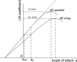
Equation 3.25 indicates that a 3D wing will produce αeff at an attitude when the aerofoil is at the angle of attack, α. Because αeff is always less than α, the wing produces less CL corresponding to aerofoil Cl (see Figure 3.28). This section describes
74 |
Aerodynamic Considerations |
Figure 3.27. Lift-curve-slope correction for aspect ratio
how to correct the 2D aerofoil data to obtain the 3D wing lift coefficient, CL, versus the angle of attack, α, relationship. Within the linear variation, dCL/dα needs to be evaluated at low angles (e.g., from −2 to 8 deg).
The 2D aerofoil lift-curve slope a0 = (dCL/dα), |
(3.32) |
where α = angle of attack (incidence).
The 2D aerofoil will generate the same lift at a lower α of αeff (see Equation 3.25) than what the wing will generate at α (α3D > α2D). Therefore, using the 2D aerofoil data, the wing lift coefficient CL can be worked at the angle of attack, α, as shown here (all angles are in degrees). The wing lift at an angle of attack, α, is as
follows: |
|
CL = a0 × αeff + constant = a0 × (α − ε) + constant |
(3.33) |
or |
|
CL = a0 × (α − 57.3CL/eµ/ AR) + constant |
|
or |
|
CL + (57.3 CL × a0/eµAR) = a0 × α + constant |
|
or |
|
CL = (a0 × α)/[1 + (57.3 × a0/eµAR)] + constant/[1 + (57.3 × a0/eµAR] |
(3.34) |
Differentiating with respect to α, it becomes: |
|
dCL/dα = a0/[1 + (57.3/eµAR)] = a = lift – curve slope of the wing |
(3.35) |
The wing tip effect delays the stall by a few degrees because the outer-wing flow distortion reduces the local angle of attack; it is shown as αmax. Note that αmax is the shift of CLmax; this value αmax is determined experimentally. In this book, the empirical relationship of αmax = 2 deg, for AR > 5 to 12, αmax = 1 deg, for AR > 12 to 20, and αmax = 0 deg, for AR > 20.
Evidently, the wing-lift-curve slope, dCL/dα = a, is less than the 2D aerofoil- lift-curve slope, a0. Figure 3.27 shows the degradation of the wing-lift-curve slope, dCL/dα, from its 2D aerofoil value.
3.15 Aspect Ratio Correction of 2D Aerofoil Characteristics for 3D Finite Wing |
75 |
Figure 3.28. Effect of t/c on dCL/dα
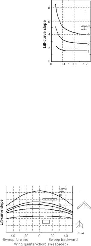
The 2D test data offer the advantage of representing any 3D wing when corrected for its aspect ratio. The effect of the wing sweep and aspect ratio on dCL/dα is shown in Figures 3.28 and 3.29 (taken from NASA).
If the flight Re is different from the experimental Re, then the correction for CLmax must be made using linear interpolation. In general, experimental data provide CLmax for several Res to facilitate interpolation and extrapolation.
Example: Given the NACA 2412 aerofoil data (see test data in Appendix D), construct wing CL versus α graph for a rectangular wing planform of aspect ratio 7 having an Oswald’s efficiency factor, e = 0.75, at a flight Re = 1.5 × 10⁶.
From the 2D aerofoil test data at Re = 6 × 10⁶, find dCl/dα = a0 = 0.095 per degree (evaluate within the linear range: −2 to 8 deg). Clmax is at α = 16 deg.
Use Equation 3.26 to obtain the 3D wing-lift-curve slope:
dCL/dα = a = a0/[1 + (57.3/eµ AR)] = 0.095/[1 + (57.3/0.75 × 3.14 × 7)]
= 0.095/1.348 = 0.067
From the 2D test data, Clmax for three Res for smooth aerofoils and one for a rough surface, interpolation results in a wing Clmax = 1.25 at flight
Figure 3.29. Effect of sweep on dCL/dα

76 |
Aerodynamic Considerations |
Figure 3.30. Wing planform definition (half wing shown)
Re = 1.5 × 10⁶. Finally, for AR = 7, the αmax increment is 1 deg, which means that the wing is stalling at (16 + 1) = 17 deg.
The wing has lost some lift-curve slope (i.e., less lift for the same angle of attack) and stalls at a slightly higher angle of attack compared to the 2D test data. Draw a vertical line from the 2D stall αmax + 1 deg (the point where the wing maximum lift is reached). Then, draw a horizontal line with CLmax = 1.25. Finally, translate the 2D stalling characteristic of α to the 3D wing-lift-curve slope joining the portion to the CLmax point following the test-data pattern.
This demonstrates that the wing CL versus the angle of attack, α, can be constructed (see Figure 3.27).
3.16 Wing Definitions
This section defines the parameters used in wing design and explains their role. The parameters are the wing planform area (also known as the wing reference area, SW); wing-sweep angle, ; and wing taper ratio, λ (dihedral and twist angles are given after the reference area is established). Also, the reference area generally does not include any extension area at the leading and trailing edges. Reference areas are concerned with the projected rectangular/trapezoidal area of the wing.
3.16.1 Planform Area, SW
The wing planform area acts as a reference area for computational purposes. The wing planform reference area is the projected area, including the area buried in the fuselage shown as a dashed line in Figure 3.30. However, the definition of the wing planform area differs among manufacturers. In commercial transport aircraft design, there are primarily two types of definitions practiced (in general) on either side of the Atlantic. The difference in planform area definition is irrelevant as long as the type is known and adhered to. This book uses the first type (Figure 3.30a), which is prevalent in the United States and has straight edges extending to the fuselage centerline. Some European definitions show the part buried inside the fuselage