are interrelated by fixed angles. This book uses the chord line for the pitch reference line as shown by the pitch angle, β, in Figure 10.30; this gives pitch, p = 2π r tanβ.

Because the blade linear velocity ωr varies with the radius, the pitch angle needs to be varied as well to make the best use of the blade-element aerofoil characteristics. When β is varied such that the pitch is not changed along the radius, then the blade has constant pitch. This means that β decreases with increases in r (the variation in β is about 40 deg from root to tip). The blade angle of attack is:

This results in an analog nondimensional parameter, J = advance ratio = V/(nD) = π tanϕ.

10.10.2 Propeller Theory

The fundamentals of propeller performance start with the idealized consideration of momentum theory. Its practical application in the industry is based on the subsequent “blade-element” theory. Both are presented in this section, followed by engineering considerations appropriate to aircraft designers. Industrial practices still use a propeller that is supplied by the manufacturer and wind-tunnel–tested generic charts and tables to evaluate its performance. Of the various forms of propeller charts, two are predominant: the NACA method and the Hamilton Standard (i.e., propeller manufacturer) method. This book prefers the Hamilton Standard method used in the industry ([16]). For designing advanced propellers and propfans to operate at speeds greater than Mach 0.6, CFD is important for arriving at the best compromise, substantiated by wind-tunnel tests. CFD employs more advanced theories (e.g., vortex theory).

Momentum Theory: Actuator Disc

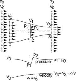
The classical incompressible inviscid momentum theory provides the basis for propeller performance ([21]). In this theory, the propeller is represented by a thin actuator disc of area, A, placed normal to the free-stream velocity, V0. This captures a stream tube within a CV that has a front surface sufficiently upstream represented by subscript “0” and sufficiently downstream represented by subscript “3” (Figure 10.33). It is assumed that thrust is uniformly distributed over the disc and the tip effects are ignored. Whether or not the disc is rotating is irrelevant because flow through it is taken without any rotation. The station numbers just in front and aft of the disc are designated as 1 and 2.

The impulse given by the disc (i.e., propeller) increases the velocity from the free-stream value of V0, smoothly accelerates to V2 behind the disc, and continues to accelerate to V3 (i.e., Station 3) until the static pressure equals the ambient pressure, p0. The pressure and velocity distribution along the stream tube is shown in Figure 10.33. There is a jump in static pressure across the disc (from p1 to p2), but there is no jump in velocity change.

Newton’s law states that the rate of change of momentum is the applied force; in this case, it is the thrust, T. Consider Station 2 of the stream tube immediately behind the disc that produces the thrust. It has a mass flow rate, m˙ = ρAdiscV2, and

Figure 10.33. Control volume showing the stream tube of the actuator disc

the change of velocity is V = (V3 – V0). This is the reactionary thrust experienced at the disc through the pressure difference multiplied by its area, A.

Thrust produced by the disc T = the rate of the change of momentum = m˙ V

=ρ Adisc × (V3 − V0)×V2

=pressure across the disc × Adisc

Equation 10.23 now can be rewritten as:

The incompressible flow in Bernoulli’s equation cannot be applied through the disc imparting the energy. Instead, two equations are set up: one for conditions ahead of and the other aft of the disc. Ambient pressure, p0, is the same everywhere.

Ahead of the disc:

Because there is no jump in velocity across the disc, the last term is omitted. Next, substitute the value of (p2 – p1) from Equation 10.24 in Equation 10.25:

This means that half of the added velocity, V/2, is ahead of the disc and the remainder, V/2, is added aft of the disc.

Using Equations 10.29 and 10.30, thrust Equation 10.23 can be rewritten as:

Applying this to an aircraft, V0 may be seen as the aircraft velocity, V, by dropping the subscript “0”. Then, the useful work rate (power, P) on the aircraft is:

For the ideal flow without the tip effects, the mechanical work produced in the system is the power, Pideal, generated to drive the propeller force (thrust, T) times velocity, V1, at the disc.

The real effects have viscous, propeller tip effects and other installation effects. In other words, to produce the same thrust, the system must provide more power (for a piston engine, it is seen as the BHP, and for a turboprop, the ESHP), where ESHP is the equivalent SHP that converts the residual thrust at the exhaust nozzle to HP, dividing by an empirical factor of 2.5. The propulsive efficiency as given in Equation 10.4 can be written as:

This gives:

ηp/ηi = {(TV)/[BHP or SHP]}/{1/[1 + ( V/2V)]}

= {(TV)[1 + ( V/2V)]/[BHP or SHP]} = 85 to 86% (typically) (10.36)

Blade-Element Theory

The practical application of propellers is obtained through blade-element theory, as described herein. A propeller-blade cross-sectional profile has the same functions as that of a wing aerofoil – that is, to operate at the best L/D.

Figure 10.30 shows that a blade-element section, dr, at radius r, is valid for any number of blades at any radius, r. Because blades are rotating elements, their properties vary along the radius.

Figure 10.30 is a velocity diagram showing that an aircraft with a flight speed of V with the propeller rotating at n rps makes the blade element advance in a helical manner. VR is the relative velocity to the blade with an angle of attack α. Here, β is the propeller pitch angle, as defined previously. Strictly speaking, each blade rotates in the wake (i.e., downwash) of the previous blade, but the current treatment ignores this effect and uses propeller charts without appreciable error.

Figure 10.30 is the force diagram of the blade element in terms of lift, L, and drag, D, that is normal and parallel, respectively, to VR. Then, the thrust, T, and force, F (producing torque), on the blade element can be obtained easily by decomposing lift and drag in the direction of flight and in the plane of the propeller rotation, respectively. Integrating this over the entire blade length (i.e., nondimensionalized as r/R – an advantage applicable to different sizes) gives the thrust, T, and torqueproducing force, F, of the blade. The root of the hub (with or without spinner) does not produce thrust, and integration is typically carried out from 0.2 to the tip, 1.0, in terms of r/R. When multiplied by the number of blades, N, this gives the propeller performance.

Therefore, propeller thrust:

By definition, advance ratio: J = V/(nD)

It has been found that from 0.7r (i.e., tapered propeller) to 0.75r (i.e., square propeller), the blades provide the aerodynamic average value that can be applied uniformly over the entire radius to obtain the propeller performance.

It also can be shown that the thrust-to-power ratio is best when the blade element works at the highest lift-to-drag ratio (L/Dmax). It is clear that a fixed-pitch blade works best at a particular aircraft speed for the given power rating (i.e., rpm) – typically, the climb condition is matched for the compromise. For this reason, constant-speed, variable-pitch propellers have better performance over a wider speed range. It is convenient to express thrust and torque in nondimensional form, as follows. From the dimensional analysis (note that the denominator omits the 1/2):

Nondimensional thrust,

TC = Thrust/(ρ V2 D2)

where σ = ambient density ratio for altitude performance Nondimensional force (for torque), TF = F/(ρ V2 D2) Force coefficient:

Therefore, torque:

Q = force × distance = Fr = CF × (ρn2 D4) × D/2

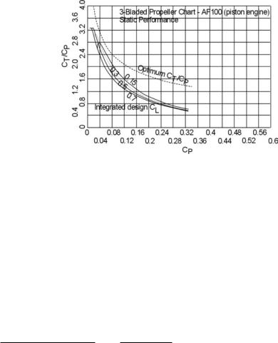
Figure 10.34. Static performance: three bladed propeller performance chart – AF100 (for a piston engine)

The wider the blade, the higher the power absorbed to a point when any further increase would offer diminishing returns in increasing thrust. A nondimensional number, defined as the total activity factor (TAF) = N × (105/16)

(r/R)3(b/D)d(r/R), expresses the integrated capacity of the blade element to absorb power. This indicates that an increase in the outward blade width is more effective than at the hub direction.

A piston engine or a gas turbine drives the propeller. Propulsive efficiency ηp can be computed by using Equations 10.35, 10.39, and 10.44.

Propulsive efficiency,

The theory determines that geometrically similar propellers can be represented in a single nondimensional chart (i.e., propeller graph) combining the nondimensional parameters, as shown in Figures 10.34 and 10.35 (for three-bladed propellers) and Figures 10.36 and 10.37 (for four-bladed propellers). Considerable amount of

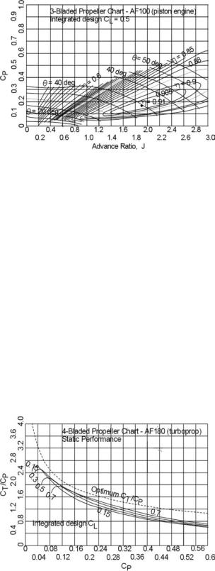
Figure 10.35. Three-bladed propeller performance chart – AF100 (for a piston engine)

coursework can be conducted using these graphs. These graphs and the procedures to estimate propeller performances are from [16], a courtesy of Hamilton Standard. These graphs are replotted retaining maximum fidelity. The reference provides the full range of graphs for other types of propellers and charts for propellers with a higher activity factor (AF).

Static computation is problematic when V is zero; then ηp = 0. Different sets of graphs are required to obtain the values of (CT/CP) to compute the takeoff thrust, as shown in Figures 10.34 and 10.36. Finally, Figure 10.38 is intended for selecting the design CL for the propeller to avoid compressibility loss. Thrust for takeoff performance can be obtained from the following equations in FPS:

In flight, thrust:

For static performance (takeoff):

Figure 10.36. Four-bladed propeller performance chart – AF180 (for a highperformance turboprop)