Davis W.A.Radio frequency circuit design.2001

130 CLASS A AMPLIFIERS

borderline between stability and instability is found from Eq. (7.17) and (7.19) when j ij D 1:

1 LS22

This equation can be squared and then split up into its complex conjugate pairs:

Substitution of Eq. (7.37) into Eq. (7.36) upon simplification yields the following factored form:

132 CLASS A AMPLIFIERS

transmission line were connected directly to the output port of the two-port circuit, then L D 0. This load would be located in the center of the Smith chart. Under this condition, Eq. (7.17) indicates that i D S11. If the known value of jS11j < 1, then j ij < 1 when the load is at the center of the Smith chart. If one point on one side of the stability circle is known to be stable, then all points on that side of the stability circle are also stable. The same rule would apply to the generator side when it is replaced by a matched load D Z0.

Unconditional stability requires that both j ij < 1 and j oj < 1 for any passive load and generator impedance attached to the ports. In this case, if jS11j < 1 and jS22j < 1, the stability circles would lie completely outside the Smith chart. Conditional stability occurs when at least one of the stability circles intersects the Smith chart. As long as the load and source impedances are on the stable side of the stability circle, stable operation occurs. This choice may not, and usually will not, coincide with the generator and load impedance for maximum transducer power gain as given by Eqs. (7.26) and (7.27). Avoiding unstable operation will usually require compromising the maximum gain for a slightly smaller but often acceptable gain. Clearly, using an impedance too close to the edge of the stability circle can result in unstable operation because of manufacturing tolerances.

7.6.2Rollett Criteria for Unconditional Stability

It is often useful to determine if a given transistor is unconditionally stable for any pair of passive impedances terminating the transistor. The two conditions necessary for this are known as the Rollett stability criteria [3] and are given as follows:

Rollett’s original derivation was done using any one of the volt–ampere immittance parameters, z, y, h, or g. Subsequently his stability equations were expressed in terms of S parameters as shown in Eqs. (7.43) and (7.44). Others arrived at stability conditions that appeared different from these, but it was pointed out that most of these alternate formulations were equivalent to those in Eqs. (7.43) and (7.44) [4]. The derivation of these two quantities will be given in this section.

The first of these equations is based on unconditional stability occurring when the load stability circle lies completely outside the Smith chart when jS11j < 1, that is,

134 CLASS A AMPLIFIERS

The original inequality, Eq. (7.50), written in terms of these new variables is

By first squaring both sides and then canceling terms, Eq. (7.59) can be greatly simplified:

Since the value of k is symmetrical on interchange of ports 1 and 2, the same result would occur with the generator port stability circle.

The second condition for unconditional stability, Eq. (7.44) can also be demonstrated based on the requirement that the j ij < 1. The second term of the right-hand side of Eq. (7.17) can be modified by multiplying it by 1 (D S22/S22) and adding 0 (D S12S21 S12S21) to the numerator. This results in the following:

set to 1. As described in [5], the quantity

1

1 jS22jej)

136 CLASS A AMPLIFIERS

When Eqs. (7.63) and (7.64) are added together,

When the term jS12S21j in Eq. (7.66) is replaced with something larger as given in Eq. (7.65), the inequality is still true:

7.6.3Stabilizing a Transistor Amplifier

There are a variety of approaches to stabilizing an amplifier. In Section 7.6.1 it was suggested that stability could be achieved from a potentially unstable transistor by making sure that the chosen amplifier terminating impedances remain inside the stable regions at all frequencies as determined by the stability circles.

Another method would be to load the amplifier with an additional shunt or series resistor on either the generator or load side. The resistor is incorporated as part of the two-port parameters of the transistor. If the condition for unconditional stability is achieved for this expanded transistor model, then optimization can be performed for the other circuit elements to achieve the desired gain and bandwidth. It is usually better to try loading the output side rather than the input side in order to minimize increasing the amplifier noise figure.

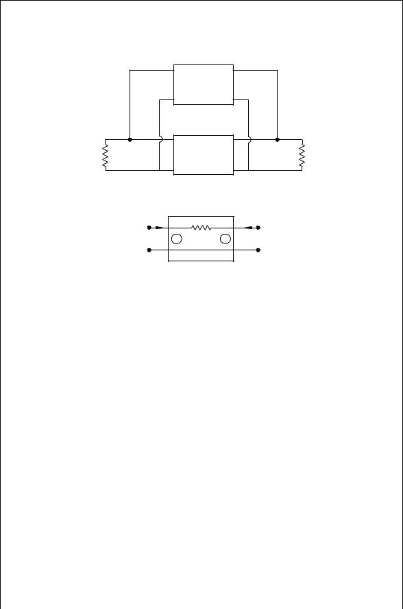
A third approach that is sometimes useful is to introduce an external feedback path that can neutralize the internal feedback of the transistor. The most widely used scheme is the shunt–shunt feedback circuit shown in Fig. 7.9. The y parameters for the composite circuit are simply the sum of the y parameters of the amplifier and feedback two-port circuits:

STABILITY 137

Feed back

Circuit

FIGURE 7.9 Shunt–shunt feedback for stabilizing a transistor.

To use this method, the transistor scattering parameters must be converted to admittance parameters (Appendix D). The y parameters for a simple series admittance, yfb can be found from circuit theory (Fig. 7.10):

If y12c could be made to be zero, then S12c would also be zero and unconditional stability could be achieved:

Since the circuit parameter g12a < 0, the value gfb < 0 must be true also. Since it is not possible to have a negative passive conductance, complete removal of

138 CLASS A AMPLIFIERS

the internal feedback is not possible. However, the susceptance, b12a, can be canceled by a passive external feedback susceptance. Although total removal of y12a cannot be achieved, yet progress toward stabilizing the amplifier can often be achieved. There is no guarantee that neutralization will provide a composite y matrix that is unconditionally stable. In addition neutralization of the feedback susceptance occurs at only one frequency.

As an example consider a transistor to have the following S parameters at a given frequency:

S11a D 0.736 102°

S21a D 2.216104°

7.78

S12a D 0.10648°

S22a D 0.476 48°

For this transistor, k D 0.752 and j j D 0.294 as found from Eqs. (7.43) and (7.44). Conversion of Eq. (7.78) to y parameters gives

y11a D 5.5307 Ð 10 3 C j1.9049 Ð 10 2 S

y12a D 3.9086 Ð 10 4 j2.3092 Ð 10 3 S

7.79

y21a D 4.7114 Ð 10 2 j2.1376 Ð 10 2 S

y22a D 5.4445 Ð 10 3 C j5.1841 Ð 10 3 S.

Nothing can be done about g12a, but b12a can be removed by setting bfb D b12a D2.3092. The composite admittance matrix becomes

y11c D 5.5307 Ð 10 3 C j1.6739 Ð 10 2 S

y12c D 3.9086 Ð 10 4 j 0 S

7.80

y21c D 4.7114 Ð 10 2 j1.9067 Ð 10 2 S

y22c D 5.4445 Ð 10 3 C j2.8750 Ð 10 3 S

The composite scattering parameters can now be found and the stability factor calculated yielding k D 2.067 and j j D 0.4037. The transistor with the feedback circuit is unconditionally stable at the given frequency. This stability has been achieved by adding inductive susceptance in shunt with the transistor input and output ports.

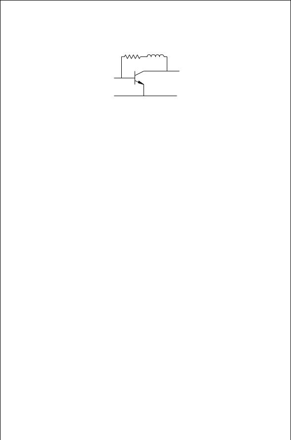
Broadband stability can be achieved by replacing the feedback inductor with an inductor and resistor as shown in Fig. 7.11. A starting value for the inductor can be found as described for the single frequency analysis. The resistor is typically in the 200 to 800 $ range, but optimum values for R and L are best found by computer optimization.

R L

FIGURE 7.11 Broadband feedback stabilization.

7.7CLASS A POWER AMPLIFIERS

Class A amplifiers, whether for small signal or large signal operation, are intended to amplify the incoming signal in a linear fashion. This type of amplifier will not introduce significant distortion in the amplitude and phase of the signal. A linear class A power amplifier will introduce low harmonic frequency components and low intermodulation distortion (IMD). An example of intermodulation distortion can be described in terms of a double sideband suppressed carrier wave, which is represented as

where ωc is the high-frequency carrier frequency and ωm is the low-frequency modulation frequency. Intermodulation distortion would result in frequencies at ωc š nωm, and harmonic distortion would cause frequency generation at kωc š nωm. The later harmonic distortion can usually be filtered out, but the intermodulation distortion is more difficult to handle because the distortion frequencies are near if not actually inside the system pass band. Clearly, this distortion in a class A amplifier is a greater problem for power amplifiers than for small signal amplifiers. Reduction of IMD depends on efficient power combining methods and careful design of the transistors themselves.

A transistor acting in the class A mode remains in its active state throughout the complete cycle of the signal. Two examples of common emitter class A amplifiers are shown in Fig. 7.12. The maximum efficiency of the class A amplifier in Fig. 7.12a has been shown to be 25%, for example [6]. However, if an RF coil can be used in the collector (Fig. 7.12b), the efficiency can be increased to almost 50%. This can be shown by recognizing first that there is no ac current flow in the bias source and no dc current flow in the load, RL. The total current flowing in the transistor collector is

and the total collector voltage is