Добавил:
Опубликованный материал нарушает ваши авторские права? Сообщите нам.
Вуз: Предмет: Файл:

Mankiw Principles of Economics (3rd ed)

.pdf
Скачиваний:
1113
Добавлен:
22.08.2013
Размер:
5.93 Mб
Скачать

400

PART SIX THE ECONOMICS OF LABOR MARKETS


VALUE OF THE


MARGINAL PRODUCT

MARGINAL PRODUCT


MARGINAL


LABOR

OUTPUT

OF LABOR

OF LABOR

WAGE

PROFIT


L


Q

MPL Q/L


PROFIT


(NUMBER OF WORKERS) (BUSHELS PER WEEK)

(BUSHELS PER WEEK)

VMPL P MPL

W

VMPL W

0

0

100

$1,000

$500

$500


1

100


80

800

500

300


2

180


60

600

500

100


3

240


40

400

500

100

4

280

20

200

500

300

5

300


HOW THE COMPETITIVE FIRM DECIDES HOW MUCH LABOR TO HIRE


Table 18-1


apples minus the total cost of producing them. The firm’s supply of apples and its


demand for workers are derived from its primary goal of maximizing profit.


THE PRODUCTION FUNCTION AND THE


MARGINAL PRODUCT OF LABOR


To make its hiring decision, the firm must consider how the size of its workforce


affects the amount of output produced. In other words, it must consider how the


number of apple pickers affects the quantity of apples it can harvest and sell. Ta-


ble 18-1 gives a numerical example. In the first column is the number of workers.


In the second column is the quantity of apples the workers harvest each week.


These two columns of numbers describe the firm’s ability to produce. As we

production function


noted in Chapter 13, economists use the term production function to describe the

the relationship between the quantity


relationship between the quantity of the inputs used in production and the quan-

of inputs used to make a good and


tity of output from production. Here the “input” is the apple pickers and the “out-

the quantity of output of that good


put” is the apples. The other inputs—the trees themselves, the land, the firm’s


trucks and tractors, and so on—are held fixed for now. This firm’s production


function shows that if the firm hires 1 worker, that worker will pick 100 bushels


of apples per week. If the firm hires 2 workers, the two workers together will pick


180 bushels per week, and so on.


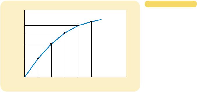
Figure 18-2 graphs the data on labor and output presented in Table 18-1. The


number of workers is on the horizontal axis, and the amount of output is on the


vertical axis. This figure illustrates the production function.


One of the Ten Principles of Economics introduced in Chapter 1 is that rational


people think at the margin. This idea is the key to understanding how firms decide


what quantity of labor to hire. To take a step toward this decision, the third column

mar ginal product


in Table 18-1 gives the marginal product of labor, the increase in the amount of

of labor


output from an additional unit of labor. When the firm increases the number of

the increase in the amount of output


workers from 1 to 2, for example, the amount of apples produced rises from 100 to

from an additional unit of labor


180 bushels. Therefore, the marginal product of the second worker is 80 bushels.


CHAPTER 18 THE MARKETS FOR THE FACTORS OF PRODUCTION

401

Quantity


of Apples


300


Production


function

280


240


180


100


0

1

2

3

4

5

Quantity of


Apple Pickers

Figure 18-2

THE PRODUCTION FUNCTION.

The production function is the relationship between the inputs into production (apple pickers) and the output from production (apples). As the quantity of the input increases, the production function gets flatter, reflecting the property of diminishing marginal product.

Notice that as the number of workers increases, the marginal product of labor declines. As you may recall from Chapter 13, this property is called diminishing marginal product. At first, when only a few workers are hired, they pick apples from the best trees in the orchard. As the number of workers increases, additional workers have to pick from the trees with fewer apples. Hence, as more and more workers are hired, each additional worker contributes less to the production of apples. For this reason, the production function in Figure 18-2 becomes flatter as the number of workers rises.

THE VALUE OF THE MARGINAL PRODUCT

AND THE DEMAND FOR LABOR

Our profit-maximizing firm is concerned more with money than with apples. As a result, when deciding how many workers to hire, the firm considers how much profit each worker would bring in. Because profit is total revenue minus total cost, the profit from an additional worker is the worker’s contribution to revenue minus the worker’s wage.

To find the worker’s contribution to revenue, we must convert the marginal product of labor (which is measured in bushels of apples) into the value of the marginal product (which is measured in dollars). We do this using the price of apples. To continue our example, if a bushel of apples sells for $10 and if an additional worker produces 80 bushels of apples, then the worker produces $800 of revenue.

The value of the marginal product of any input is the marginal product of that input multiplied by the market price of the output. The fourth column in Table 18-1 shows the value of the marginal product of labor in our example, assuming the price of apples is $10 per bushel. Because the market price is constant for a competitive firm, the value of the marginal product (like the marginal product itself) diminishes as the number of workers rises.

diminishing mar ginal product

the property whereby the marginal product of an input declines as the quantity of the input increases

value of the mar ginal product

the marginal product of an input times the price of the output

402

PART SIX THE ECONOMICS OF LABOR MARKETS

Figure 18-3

THE VALUE OF THE MARGINAL

PRODUCT OF LABOR. This figure shows how the value of the marginal product (the marginal product times the price of the output) depends on the number of workers. The curve slopes downward because of diminishing marginal product. For a competitive, profitmaximizing firm, this value-of- marginal-product curve is also the firm’s labor demand curve.

Value

of the

Marginal

Product

Market

wage

Value of marginal product

(demand curve for labor)

0

Profit-maximizing quantity

Quantity of


Apple Pickers

Now consider how many workers the firm will hire. Suppose that the market wage for apple pickers is $500 per week. In this case, the first worker that the firm hires is profitable: The first worker yields $1,000 in revenue, or $500 in profit. Similarly, the second worker yields $800 in additional revenue, or $300 in profit. The third worker produces $600 in additional revenue, or $100 in profit. After the third worker, however, hiring workers is unprofitable. The fourth worker would yield only $400 of additional revenue. Because the worker’s wage is $500, hiring the fourth worker would mean a $100 reduction in profit. Thus, the firm hires only three workers.

It is instructive to consider the firm’s decision graphically. Figure 18-3 graphs the value of the marginal product. This curve slopes downward because the marginal product of labor diminishes as the number of workers rises. The figure also includes a horizontal line at the market wage. To maximize profit, the firm hires workers up to the point where these two curves cross. Below this level of employment, the value of the marginal product exceeds the wage, so hiring another worker would increase profit. Above this level of employment, the value of the marginal product is less than the wage, so the marginal worker is unprofitable. Thus, a competitive, profit-maximizing firm hires workers up to the point where the value of the marginal product of labor equals the wage.

Having explained the profit-maximizing hiring strategy for a competitive firm, we can now offer a theory of labor demand. Recall that a firm’s labor demand curve tells us the quantity of labor that a firm demands at any given wage. We have just seen in Figure 18-3 that the firm makes that decision by choosing the quantity of labor at which the value of the marginal product equals the wage. As a result, the value-of-marginal-product curve is the labor demand curve for a competitive, profit-maximizing firm.


CHAPTER 18 THE MARKETS FOR THE FACTORS OF PRODUCTION

403


F Y I


Input Demand

In Chapter 14 we saw how

worker adds less to the production of apples (MPL falls).

and Output

a competitive, profit-maximizing

Similarly, when the apple firm is producing a large quantity

Supply: Two

firm decides how much of its

of apples, the orchard is already crowded with workers, so it

Sides of the

output to sell: It chooses the

is more costly to produce an additional bushel of apples

Same Coin

quantity of output at which the

(MC rises).


price of the good equals the

Now consider our criterion for profit maximization. We


marginal cost of production. We

determined earlier that a profit-maximizing firm chooses the


have just seen how such a firm

quantity of labor so that the value of the marginal product


decides how much labor to

(P MPL) equals the wage (W). We can write this mathe-


hire: It chooses the quantity of

matically as


labor at which the wage equals


the value of the marginal prod-

P MPL W.


uct. Because the production

If we divide both sides of this equation by MPL, we obtain


function links the quantity of inputs to the quantity of output,


you should not be surprised to learn that the firm’s decision


about input demand is closely linked to its decision about

P W/MPL.


output supply. In fact, these two decisions are two sides of


the same coin.


We just noted that W/MPL equals marginal cost MC. There-

To see this relationship more fully, let’s consider how

fore, we can substitute to obtain


the marginal product of labor (MPL) and marginal cost (MC)


are related. Suppose an additional worker costs $500 and

P MC.


has a marginal product of 50 bushels of apples. In this


case, producing 50 more bushels costs $500; the marginal

This equation states that the price of the firm’s output is

cost of a bushel is $500/50, or $10. More generally, if W

equal to the marginal cost of producing a unit of output.

is the wage, and an extra unit of labor produces MPL units

Thus, when a competitive firm hires labor up to the point at

of output, then the marginal cost of a unit of output is

which the value of the marginal product equals the wage, it

MC W/MPL.


also produces up to the point at which the price equals mar-

This analysis shows that diminishing marginal product

ginal cost. Our analysis of labor demand in this chapter is

is closely related to increasing marginal cost. When our ap-

just another way of looking at the production decision we

ple orchard grows crowded with workers, each additional

first saw in Chapter 14.


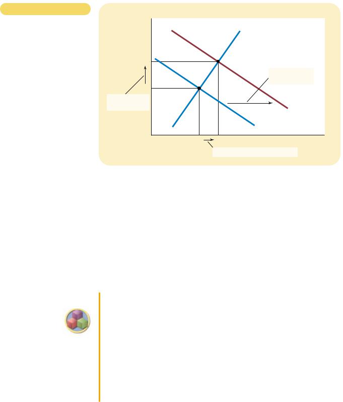
WHAT CAUSES THE LABOR DEMAND CURVE TO SHIFT?

We now understand the labor demand curve: It is nothing more than a reflection of the value of marginal product of labor. With this insight in mind, let’s consider a few of the things that might cause the labor demand curve to shift.

The Output Price The value of the marginal product is marginal product times the price of the firm’s output. Thus, when the output price changes, the value of the marginal product changes, and the labor demand curve shifts. An increase in the price of apples, for instance, raises the value of the marginal product of each worker that picks apples and, therefore, increases labor demand from the firms that supply apples. Conversely, a decrease in the price of apples reduces the value of the marginal product and decreases labor demand.

Technological Change Between 1968 and 1998, the amount of output a typical U.S. worker produced in an hour rose by 57 percent. Why? The most

404

PART SIX THE ECONOMICS OF LABOR MARKETS

important reason is technological progress: Scientists and engineers are constantly figuring out new and better ways of doing things. This has profound implications for the labor market. Technological advance raises the marginal product of labor, which in turn increases the demand for labor. Such technological advance explains persistently rising employment in face of rising wages: Even though wages (adjusted for inflation) increased by 62 percent over these three decades, firms nonetheless increased by 72 percent the number of workers they employed.

The Supply of Other Factors The quantity available of one factor of production can affect the marginal product of other factors. A fall in the supply of ladders, for instance, will reduce the marginal product of apple pickers and thus the demand for apple pickers. We consider this linkage among the factors of production more fully later in the chapter.

QUICK QUIZ: Define marginal product of labor and value of the marginal product of labor. Describe how a competitive, profit-maximizing firm decides how many workers to hire.

THE SUPPLY OF LABOR

Having analyzed labor demand in detail, let’s turn to the other side of the market and consider labor supply. A formal model of labor supply is included in Chapter 21, where we develop the theory of household decisionmaking. Here we discuss briefly and informally the decisions that lie behind the labor supply curve.

THE TRADEOFF BETWEEN WORK AND LEISURE

One of the Ten Principles of Economics in Chapter 1 is that people face tradeoffs. Probably no tradeoff is more obvious or more important in a person’s life than the tradeoff between work and leisure. The more hours you spend working, the fewer hours you have to watch TV, have dinner with friends, or pursue your favorite hobby. The tradeoff between labor and leisure lies behind the labor supply curve.

Another one of the Ten Principles of Economics is that the cost of something is what you give up to get it. What do you give up to get an hour of leisure? You give up an hour of work, which in turn means an hour of wages. Thus, if your wage is $15 per hour, the opportunity cost of an hour of leisure is $15. And when you get a raise to $20 per hour, the opportunity cost of enjoying leisure goes up.

The labor supply curve reflects how workers’ decisions about the labor–leisure tradeoff respond to a change in that opportunity cost. An upward-sloping labor supply curve means that an increase in the wage induces workers to increase the quantity of labor they supply. Because time is limited, more hours of work means that workers are enjoying less leisure. That is, workers respond to the increase in the opportunity cost of leisure by taking less of it.

It is worth noting that the labor supply curve need not be upward sloping. Imagine you got that raise from $15 to $20 per hour. The opportunity cost of

CHAPTER 18 THE MARKETS FOR THE FACTORS OF PRODUCTION

405

leisure is now greater, but you are also richer than you were before. You might decide that with your extra wealth you can now afford to enjoy more leisure; in this case, your labor supply curve would slope backwards. In Chapter 21, we discuss this possibility in terms of conflicting effects on your labor-supply decision (called income and substitution effects). For now, we ignore the possibility of backward-sloping labor supply and assume that the labor supply curve is upward sloping.

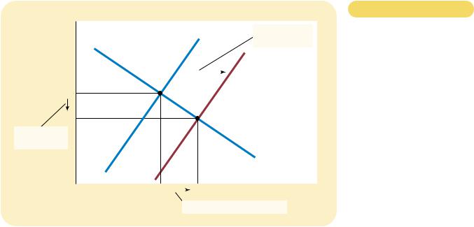
WHAT CAUSES THE LABOR SUPPLY CURVE TO SHIFT?

The labor supply curve shifts whenever people change the amount they want to work at a given wage. Let’s now consider some of the events that might cause such a shift.

Changes in Tastes In 1950, 34 percent of women were employed at paid jobs or looking for work. In 1998, the number had risen to 60 percent. There are, of course, many explanations for this development, but one of them is changing tastes, or attitudes toward work. A generation or two ago, it was the norm for women to stay at home while raising children. Today, family sizes are smaller, and more mothers choose to work. The result is an increase in the supply of labor.

Changes in Alternative Oppor tunities The supply of labor in any one labor market depends on the opportunities available in other labor markets. If the wage earned by pear pickers suddenly rises, some apple pickers may choose to switch occupations. The supply of labor in the market for apple pickers falls.

Immigration Movements of workers from region to region, or country to country, is an obvious and often important source of shifts in labor supply. When immigrants come to the United States, for instance, the supply of labor in the United States increases and the supply of labor in the immigrants’ home countries contracts. In fact, much of the policy debate about immigration centers on its effect on labor supply and, thereby, equilibrium in the labor market.

QUICK QUIZ: Who has a greater opportunity cost of enjoying leisure—a janitor or a brain surgeon? Explain. Can this help explain why doctors work such long hours?

EQUILIBRIUM IN THE LABOR MARKET

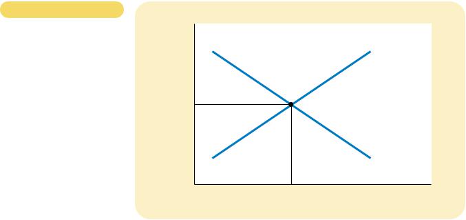
So far we have established two facts about how wages are determined in competitive labor markets:

The wage adjusts to balance the supply and demand for labor.

The wage equals the value of the marginal product of labor.

406 PART SIX THE ECONOMICS OF LABOR MARKETS

Figure 18-4

EQUILIBRIUM IN A LABOR

Wage

MARKET. Like all prices, the

(price of

labor)

price of labor (the wage) depends


on supply and demand. Because


the demand curve reflects the


value of the marginal product of


labor, in equilibrium workers

Equilibrium

receive the value of their

wage, W

marginal contribution to the


production of goods and services.


Supply

Demand

0

Equilibrium

Quantity of


employment, L

Labor

At first, it might seem surprising that the wage can do both these things at once. In fact, there is no real puzzle here, but understanding why there is no puzzle is an important step to understanding wage determination.

Figure 18-4 shows the labor market in equilibrium. The wage and the quantity of labor have adjusted to balance supply and demand. When the market is in this equilibrium, each firm has bought as much labor as it finds profitable at the equilibrium wage. That is, each firm has followed the rule for profit maximization: It has hired workers until the value of the marginal product equals the wage. Hence, the wage must equal the value of marginal product of labor once it has brought supply and demand into equilibrium.

This brings us to an important lesson: Any event that changes the supply or demand for labor must change the equilibrium wage and the value of the marginal product by the same amount, because these must always be equal. To see how this works, let’s consider some events that shift these curves.

SHIFTS IN LABOR SUPPLY

Suppose that immigration increases the number of workers willing to pick apples. As Figure 18-5 shows, the supply of labor shifts to the right from S1 to S2. At the initial wage W1, the quantity of labor supplied now exceeds the quantity demanded. This surplus of labor puts downward pressure on the wage of apple pickers, and the fall in the wage from W1 to W2 in turn makes it profitable for firms to hire more workers. As the number of workers employed in each apple orchard rises, the marginal product of a worker falls, and so does the value of the marginal product. In the new equilibrium, both the wage and the value of the marginal product of labor are lower than they were before the influx of new workers.

Wage (price of labor)

W1

W2

2. . . . reduces the wage . . .

0

CHAPTER 18 THE MARKETS FOR THE FACTORS OF PRODUCTION

407

Figure 18-5

1. An increase in

Supply, S1

labor supply . . .


S2


Demand


L1


L2

Quantity of


Labor

3. . . . and raises employment.

A SHIFT IN LABOR SUPPLY.

When labor supply increases from S1 to S2, perhaps because of an immigration of new workers, the equilibrium wage falls from W1 to W2. At this lower wage, firms hire more labor, so employment rises from L1 to L2. The change in the wage reflects a change in the value of the marginal product of labor: With more workers, the added output from an extra worker is smaller.

An episode from Israel illustrates how a shift in labor supply can alter the equilibrium in a labor market. During most of the 1980s, many thousands of Palestinians regularly commuted from their homes in the Israeli-occupied West Bank and Gaza Strip to jobs in Israel, primarily in the construction and agriculture industries. In 1988, however, political unrest in these occupied areas induced the Israeli government to take steps that, as a by-product, reduced this supply of workers. Curfews were imposed, work permits were checked more thoroughly, and a ban on overnight stays of Palestinians in Israel was enforced more rigorously. The economic impact of these steps was exactly as theory predicts: The number of Palestinians with jobs in Israel fell by half, while those who continued to work in Israel enjoyed wage increases of about 50 percent. With a reduced number of Palestinian workers in Israel, the value of the marginal product of the remaining workers was much higher.

SHIFTS IN LABOR DEMAND

Now suppose that an increase in the popularity of apples causes their price to rise. This price increase does not change the marginal product of labor for any given number of workers, but it does raise the value of the marginal product. With a higher price of apples, hiring more apple pickers is now profitable. As Figure 18-6 shows, when the demand for labor shifts to the right from D1 to D2, the equilibrium wage rises from W1 to W2, and equilibrium employment rises from L1 to L2. Once again, the wage and the value of the marginal product of labor move together.

This analysis shows that prosperity for firms in an industry is often linked to prosperity for workers in that industry. When the price of apples rises, apple

408

PART SIX THE ECONOMICS OF LABOR MARKETS

Figure 18-6

A SHIFT IN LABOR DEMAND.

When labor demand increases from D1 to D2, perhaps because of an increase in the price of the firms’ output, the equilibrium wage rises from W1 to W2, and employment rises from L1 to L2. Again, the change in the wage reflects a change in the value of the marginal product of labor: With a higher output price, the added output from an extra worker is more valuable.

Wage


(price of


Supply

labor)


W2


1. An increase in


labor demand . . .

W1


2. . . . increases


the wage . . .


D2


Demand, D1

0

L1

L2

Quantity of


Labor


3. . . . and increases employment.

producers make greater profit, and apple pickers earn higher wages. When the price of apples falls, apple producers earn smaller profit, and apple pickers earn lower wages. This lesson is well known to workers in industries with highly volatile prices. Workers in oil fields, for instance, know from experience that their earnings are closely linked to the world price of crude oil.

From these examples, you should now have a good understanding of how wages are set in competitive labor markets. Labor supply and labor demand together determine the equilibrium wage, and shifts in the supply or demand curve for labor cause the equilibrium wage to change. At the same time, profit maximization by the firms that demand labor ensures that the equilibrium wage always equals the value of the marginal product of labor.

CASE STUDY PRODUCTIVITY AND WAGES

One of the Ten Principles of Economics in Chapter 1 is that our standard of living depends on our ability to produce goods and services. We can now see how this principle works in the market for labor. In particular, our analysis of labor demand shows that wages equal productivity as measured by the value of the marginal product of labor. Put simply, highly productive workers are highly paid, and less productive workers are less highly paid.

This lesson is key to understanding why workers today are better off than workers in previous generations. Table 18-2 presents some data on growth in productivity and growth in wages (adjusted for inflation). From 1959 to 1997, productivity as measured by output per hour of work grew about 1.8 percent per year; at this rate, productivity doubles about every 40 years. Over this period, wages grew at a similar rate of 1.7 percent per year.

CHAPTER 18 THE MARKETS FOR THE FACTORS OF PRODUCTION

409


GROWTH RATE

GROWTH RATE

TIME PERIOD

OF PRODUCTIVITY

OF REAL WAGES


1959–1997

1.8

1.7

1959–1973

2.9

2.9

1973–1997

1.1

1.0


SOURCE: Economic Report of the President 1999, table B-49, p. 384. Growth in productivity is measured here as the annualized rate of change in output per hour in the nonfarm business sector. Growth in real wages is measured as the annualized change in compensation per hour in the nonfarm business sector divided by the implicit price deflator for that sector. These productivity data measure average productivity—the quantity of output divided by the quantity of labor—rather than marginal productivity, but average and marginal productivity are thought to move closely together.

Table 18-2 also shows that, beginning around 1973, growth in productivity slowed from 2.9 to 1.1 percent per year. This 1.8 percentage-point slowdown in productivity coincided with a slowdown in wage growth of 1.9 percentage points. Because of this productivity slowdown, workers in the 1980s and 1990s did not experience the same rapid growth in living standards that their parents enjoyed. A slowdown of 1.8 percentage points might not seem large, but accumulated over many years, even a small change in a growth rate is significant. If productivity and wages had grown at the same rate since 1973 as they did previously, workers’ earnings would now be about 50 percent higher than they are.

The link between productivity and wages also sheds light on international experience. Table 18-3 presents some data on productivity growth and wage growth for a representative group of countries, ranked in order of their productivity growth. Although these international data are far from precise, a close link between the two variables is apparent. In South Korea, Hong Kong, and Singapore, productivity has grown rapidly, and so have wages. In Mexico, Argentina, and Iran, productivity has fallen, and so have wages. The United States falls about in the middle of the distribution: By international standards, U.S. productivity growth and wage growth have been neither exceptionally bad nor exceptionally good.

What causes productivity and wages to vary so much over time and across countries? A complete answer to this question requires an analysis of long-run economic growth, a topic beyond the scope of this chapter. We can, however, briefly note three key determinants of productivity:

Physical capital: When workers work with a larger quantity of equipment and structures, they produce more.

Human capital: When workers are more educated, they produce more.

Technological knowledge: When workers have access to more sophisticated technologies, they produce more.

Physical capital, human capital, and technological knowledge are the ultimate sources of most of the differences in productivity, wages, and standards of living.

Table 18-2

PRODUCTIVITY AND WAGE

GROWTH IN THE UNITED STATES