Mankiw Principles of Economics (3rd ed)
.pdf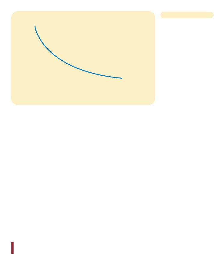
15 MONOPOLY |
319 |
|
|
|
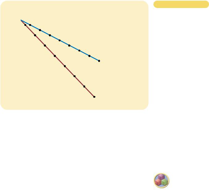
Figur e 15-1 |
|
|
|
|
Cost |
|
|
ECONOMIES OF SCALE AS A |
|
|||
|
|
|
CAUSE OF MONOPOLY. When a |
|
|
|
firm’s average-total-cost curve |
|
|
|
continually declines, the firm |
|
|
|
has what is called a natural |
|
|
|
monopoly. In this case, when |
|
|
|
production is divided among |
|
|
|
more firms, each firm produces |
|
|
|
less, and average total cost rises. |
|
|
|
As a result, a single firm can |
|
|
|
produce any given amount at |
|
Average |
|
the smallest cost. |
|
|
|
|
|
total |
|
|
|
cost |
|
|
|
|
|
|
0 |
Quantity of Output |
||
We saw other examples of natural monopolies when we discussed public goods and common resources in Chapter 11. We noted in passing that some goods in the economy are excludable but not rival. An example is a bridge used so infrequently that it is never congested. The bridge is excludable because a toll collector can prevent someone from using it. The bridge is not rival because use of the bridge by one person does not diminish the ability of others to use it. Because there is a fixed cost of building the bridge and a negligible marginal cost of additional users, the average total cost of a trip across the bridge (the total cost divided by the number of trips) falls as the number of trips rises. Hence, the bridge is a natural monopoly.
When a firm is a natural monopoly, it is less concerned about new entrants eroding its monopoly power. Normally, a firm has trouble maintaining a monopoly position without ownership of a key resource or protection from the government. The monopolist’s profit attracts entrants into the market, and these entrants make the market more competitive. By contrast, entering a market in which another firm has a natural monopoly is unattractive. Would-be entrants know that they cannot achieve the same low costs that the monopolist enjoys because, after entry, each firm would have a smaller piece of the market.
In some cases, the size of the market is one determinant of whether an industry is a natural monopoly. Consider a bridge across a river. When the population is small, the bridge may be a natural monopoly. A single bridge can satisfy the entire demand for trips across the river at lowest cost. Yet as the population grows and the bridge becomes congested, satisfying the entire demand may require two or more bridges across the same river. Thus, as a market expands, a natural monopoly can evolve into a competitive market.
QUICK QUIZ: What are the three reasons that a market might have a monopoly? Give two examples of monopolies, and explain the reason for each.
320 |
PART FIVE FIRM BEHAVIOR AND THE ORGANIZATION OF INDUSTRY |
HOW MONOPOLIES MAKE PRODUCTION
AND PRICING DECISIONS
Now that we know how monopolies arise, we can consider how a monopoly firm decides how much of its product to make and what price to charge for it. The analysis of monopoly behavior in this section is the starting point for evaluating whether monopolies are desirable and what policies the government might pursue in monopoly markets.
MONOPOLY VERSUS COMPETITION
The key difference between a competitive firm and a monopoly is the monopoly’s ability to influence the price of its output. A competitive firm is small relative to the market in which it operates and, therefore, takes the price of its output as given by market conditions. By contrast, because a monopoly is the sole producer in its market, it can alter the price of its good by adjusting the quantity it supplies to the market.
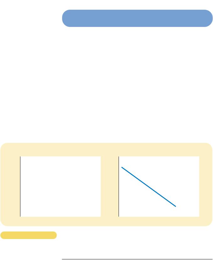
One way to view this difference between a competitive firm and a monopoly is to consider the demand curve that each firm faces. When we analyzed profit maximization by competitive firms in Chapter 14, we drew the market price as a horizontal line. Because a competitive firm can sell as much or as little as it wants at this price, the competitive firm faces a horizontal demand curve, as in panel (a) of Figure 15-2. In effect, because the competitive firm sells a product with many
(a) A Competitive Firm’s Demand Curve |
(b) A Monopolist’s Demand Curve |
Price |
Price |
|
|
Demand |
|
|
Demand |
||
|
|
|
|
||||
|
|
|
|
|
|
||
|
|
|
|
|
|
|
|
0 |
Quantity of Output |
0 |
|
Quantity of Output |
|||
|
DEMAND CURVES FOR COMPETITIVE AND MONOPOLY FIRMS. |
Because competitive firms |
|||||
Figur e 15-2
are price takers, they in effect face horizontal demand curves, as in panel (a). Because a monopoly firm is the sole producer in its market, it faces the downward-sloping market demand curve, as in panel (b). As a result, the monopoly has to accept a lower price if it wants to sell more output.

CHAPTER 15 MONOPOLY |
321 |
perfect substitutes (the products of all the other firms in its market), the demand curve that any one firm faces is perfectly elastic.
By contrast, because a monopoly is the sole producer in its market, its demand curve is the market demand curve. Thus, the monopolist’s demand curve slopes downward for all the usual reasons, as in panel (b) of Figure 15-2. If the monopolist raises the price of its good, consumers buy less of it. Looked at another way, if the monopolist reduces the quantity of output it sells, the price of its output increases.
The market demand curve provides a constraint on a monopoly’s ability to profit from its market power. A monopolist would prefer, if it were possible, to charge a high price and sell a large quantity at that high price. The market demand curve makes that outcome impossible. In particular, the market demand curve describes the combinations of price and quantity that are available to a monopoly firm. By adjusting the quantity produced (or, equivalently, the price charged), the monopolist can choose any point on the demand curve, but it cannot choose a point off the demand curve.
What point on the demand curve will the monopolist choose? As with competitive firms, we assume that the monopolist’s goal is to maximize profit. Because the firm’s profit is total revenue minus total costs, our next task in explaining monopoly behavior is to examine a monopolist’s revenue.
A MONOPOLY’S REVENUE
Consider a town with a single producer of water. Table 15-1 shows how the monopoly’s revenue might depend on the amount of water produced.
The first two columns show the monopolist’s demand schedule. If the monopolist produces 1 gallon of water, it can sell that gallon for $10. If it produces
QUANTITY |
|
|
|
|
|
OF WATER |
PRICE |
TOTAL REVENUE |
AVERAGE REVENUE |
MARGINAL REVENUE |
|
|
|
|
|
|
|
(Q) |
(P) |
(TR P Q) |
(AR TR/Q) |
(MR TR/ Q) |
|
|
|
|
|
|
|
0 gallons |
$11 |
$ 0 |
— |
$10 |
|
1 |
10 |
10 |
$10 |
||
8 |
|||||
2 |
9 |
18 |
9 |
||
6 |
|||||
3 |
8 |
24 |
8 |
||
4 |
|||||
4 |
7 |
28 |
7 |
||
2 |
|||||
5 |
6 |
30 |
6 |
||
0 |
|||||
6 |
5 |
30 |
5 |
||
2 |
|||||
7 |
4 |
28 |
4 |
||
4 |
|||||
8 |
3 |
24 |
3 |
||
|
A MONOPOLY’S TOTAL, AVERAGE, AND MARGINAL REVENUE
Table 15-1
322 |
PART FIVE FIRM BEHAVIOR AND THE ORGANIZATION OF INDUSTRY |
2 gallons, it must lower the price to $9 in order to sell both gallons. And if it produces 3 gallons, it must lower the price to $8. And so on. If you graphed these two columns of numbers, you would get a typical downward-sloping demand curve.
The third column of the table presents the monopolist’s total revenue. It equals the quantity sold (from the first column) times the price (from the second column). The fourth column computes the firm’s average revenue, the amount of revenue the firm receives per unit sold. We compute average revenue by taking the number for total revenue in the third column and dividing it by the quantity of output in the first column. As we discussed in Chapter 14, average revenue always equals the price of the good. This is true for monopolists as well as for competitive firms.
The last column of Table 15-1 computes the firm’s marginal revenue, the amount of revenue that the firm receives for each additional unit of output. We compute marginal revenue by taking the change in total revenue when output increases by 1 unit. For example, when the firm is producing 3 gallons of water, it receives total revenue of $24. Raising production to 4 gallons increases total revenue to $28. Thus, marginal revenue is $28 minus $24, or $4.
Table 15-1 shows a result that is important for understanding monopoly behavior: A monopolist’s marginal revenue is always less than the price of its good. For example, if the firm raises production of water from 3 to 4 gallons, it will increase total revenue by only $4, even though it will be able to sell each gallon for $7. For a monopoly, marginal revenue is lower than price because a monopoly faces a downward-sloping demand curve. To increase the amount sold, a monopoly firm must lower the price of its good. Hence, to sell the fourth gallon of water, the monopolist must get less revenue for each of the first three gallons.
Marginal revenue is very different for monopolies from what it is for competitive firms. When a monopoly increases the amount it sells, it has two effects on total revenue (P Q):
The output effect: More output is sold, so Q is higher.
The price effect: The price falls, so P is lower.
Because a competitive firm can sell all it wants at the market price, there is no price effect. When it increases production by 1 unit, it receives the market price for that unit, and it does not receive any less for the amount it was already selling. That is, because the competitive firm is a price taker, its marginal revenue equals the price of its good. By contrast, when a monopoly increases production by 1 unit, it must reduce the price it charges for every unit it sells, and this cut in price reduces revenue on the units it was already selling. As a result, a monopoly’s marginal revenue is less than its price.
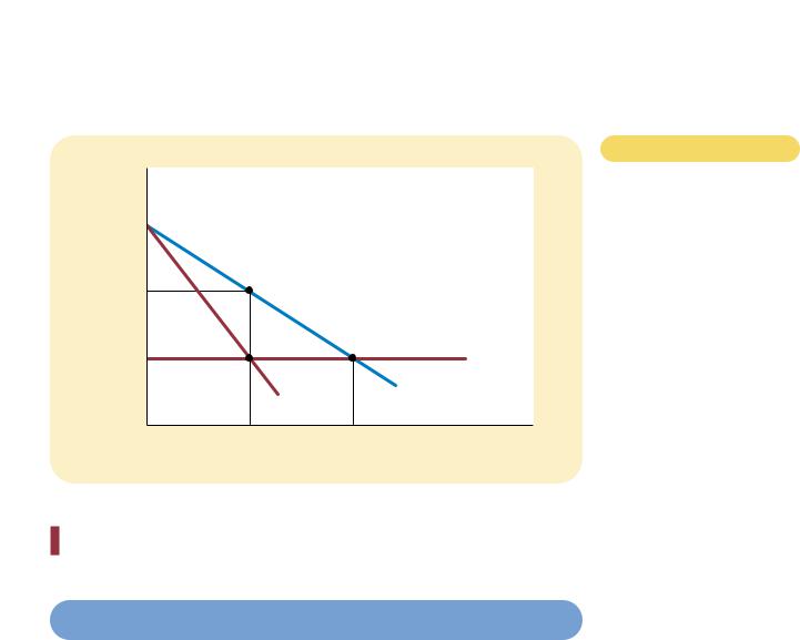
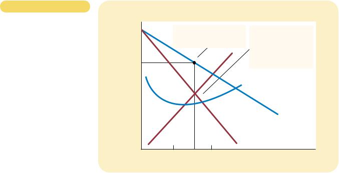
Figure 15-3 graphs the demand curve and the marginal-revenue curve for a monopoly firm. (Because the firm’s price equals its average revenue, the demand curve is also the average-revenue curve.) These two curves always start at the same point on the vertical axis because the marginal revenue of the first unit sold equals the price of the good. But, for the reason we just discussed, the monopolist’s marginal revenue is less than the price of the good. Thus, a monopoly’s marginalrevenue curve lies below its demand curve.
You can see in the figure (as well as in Table 15-1) that marginal revenue can even become negative. Marginal revenue is negative when the price effect on
 A
A
CHAPTER 15 MONOPOLY |
325 |
|
F Y I |
|
|
|
|
Why a |
|
You may have noticed that we |
tells us the quantity that firms choose to supply at any given |
|
Monopoly Does |
|
have analyzed the price in a |
price. This concept makes sense when we are analyzing com- |
|
Not Have a |
|
monopoly market using the |
petitive firms, which are price takers. But a monopoly firm is |
|
|
market demand curve and the |
a price maker, not a price taker. It is not meaningful to ask |
|
|
Supply Curve |
|
||
|
|
firm’s cost curves. We have not |
what such a firm would produce at any price because the |
|
|
|
|
||
|
|
|
made any mention of the mar- |
firm sets the price at the same time it chooses the quantity |
|
|
|
ket supply curve. By contrast, |
to supply. |
|
|
|
when we analyzed prices in |
Indeed, the monopolist’s decision about how much to |
|
|
|
competitive markets beginning |
supply is impossible to separate from the demand curve it |
|
|
|
in Chapter 4, the two most im- |
faces. The shape of the demand curve determines the |
|
|
|
portant words were always sup- |
shape of the marginal-revenue curve, which in turn deter- |
|
|
|
ply and demand. |
mines the monopolist’s profit-maximizing quantity. In a com- |
|
|
|
What happened to the sup- |
petitive market, supply decisions can be analyzed without |
|
ply curve? Although monopoly firms make decisions about |
knowing the demand curve, but that is not true in a monop- |
||
|
what quantity to supply (in the way described in this chapter), |
oly market. Therefore, we never talk about a monopoly’s |
||
|
a monopoly does not have a supply curve. A supply curve |
supply curve. |
||
|
|
|
|
|
cost, it uses the demand curve to find the price consistent with that quantity. In Figure 15-4, the profit-maximizing price is found at point B.
We can now see a key difference between markets with competitive firms and markets with a monopoly firm: In competitive markets, price equals marginal cost. In monopolized markets, price exceeds marginal cost. As we will see in a moment, this finding is crucial to understanding the social cost of monopoly.
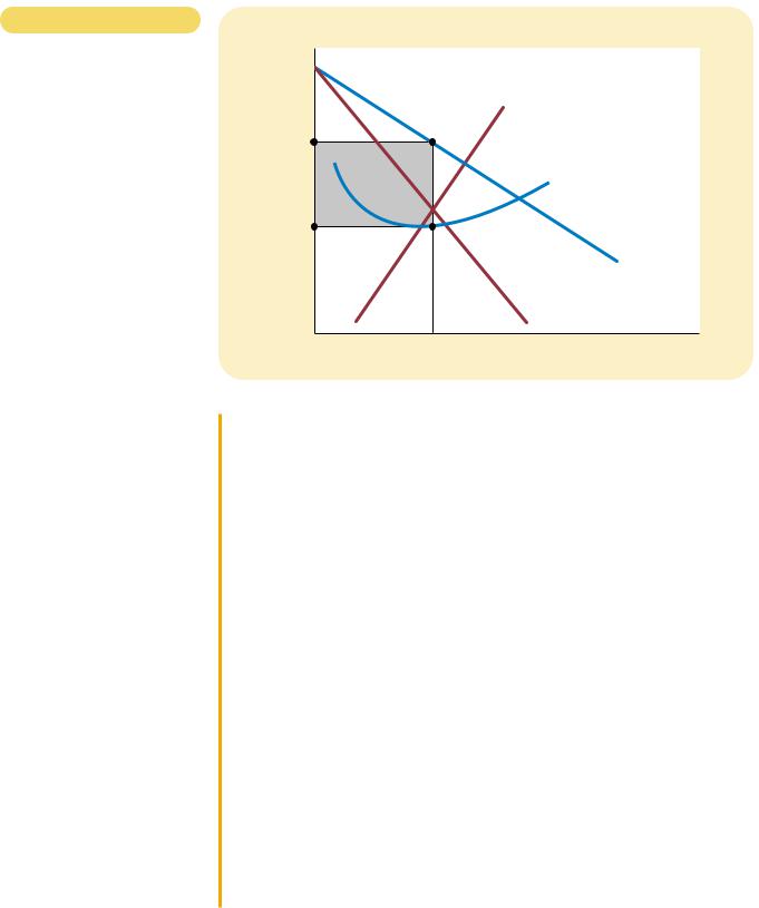
A MONOPOLY’S PROFIT
How much profit does the monopoly make? To see the monopoly’s profit, recall that profit equals total revenue (TR) minus total costs (TC):
Profit TR TC.
We can rewrite this as
Profit (TR/Q TC/Q) Q.
TR/Q is average revenue, which equals the price P, and TC/Q is average total cost
ATC. Therefore,
Profit (P ATC) Q.
This equation for profit (which is the same as the profit equation for competitive firms) allows us to measure the monopolist’s profit in our graph.
Consider the shaded box in Figure 15-5. The height of the box (the segment BC) is price minus average total cost, P – ATC, which is the profit on the typical unit sold. The width of the box (the segment DC) is the quantity sold QMAX. Therefore, the area of this box is the monopoly firm’s total profit.