CHAPTER 14 FIRMS IN COMPETITIVE MARKETS |
299 |
Costs
MC
Firm’s short-run supply curve
ATC
AVC
Firm shuts down if
P AVC
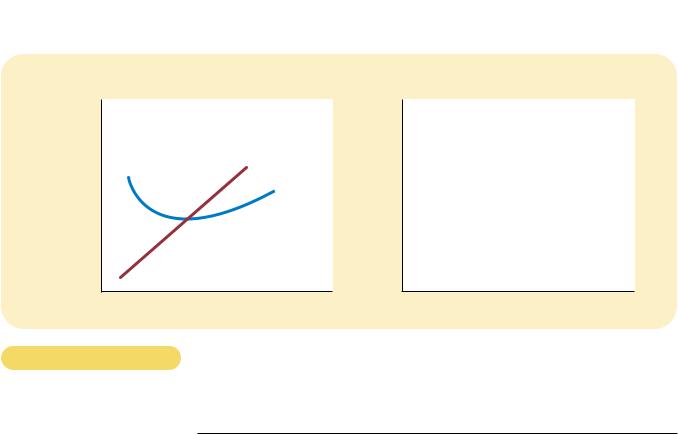
Figur e 14-3
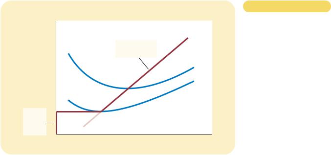
THE COMPETITIVE FIRM’S SHORT-
RUN SUPPLY CURVE. In the
short run, the competitive firm’s supply curve is its marginal-cost curve (MC) above average variable cost (AVC). If the price falls below average variable cost, the firm is better off shutting down.
do one thing instead of another, whereas a sunk cost cannot be avoided, regardless of the choices you make. Because nothing can be done about sunk costs, you can ignore them when making decisions about various aspects of life, including business strategy.
Our analysis of the firm’s shutdown decision is one example of the irrelevance of sunk costs. We assume that the firm cannot recover its fixed costs by temporarily stopping production. As a result, the firm’s fixed costs are sunk in the short run, and the firm can safely ignore these costs when deciding how much to produce. The firm’s short-run supply curve is the part of the marginal-cost curve that lies above average variable cost, and the size of the fixed cost does not matter for this supply decision.
The irrelevance of sunk costs explains how real businesses make decisions. In the early 1990s, for instance, most of the major airlines reported large losses. In one year, American Airlines, Delta, and USAir each lost more than $400 million. Yet despite the losses, these airlines continued to sell tickets and fly passengers. At first, this decision might seem surprising: If the airlines were losing money flying planes, why didn’t the owners of the airlines just shut down their businesses?
To understand this behavior, we must acknowledge that many of the airlines’ costs are sunk in the short run. If an airline has bought a plane and cannot resell it, then the cost of the plane is sunk. The opportunity cost of a flight includes only the variable costs of fuel and the wages of pilots and flight attendants. As long as the total revenue from flying exceeds these variable costs, the airlines should continue operating. And, in fact, they did.
The irrelevance of sunk costs is also important for personal decisions. Imagine, for instance, that you place a $10 value on seeing a newly released movie. You buy a ticket for $7, but before entering the theater, you lose the ticket. Should you buy another ticket? Or should you now go home and refuse to pay a total of $14 to see the movie? The answer is that you should buy another ticket. The benefit of seeing
300 |
PART FIVE FIRM BEHAVIOR AND THE ORGANIZATION OF INDUSTRY |
the movie ($10) still exceeds the opportunity cost (the $7 for the second ticket). The $7 you paid for the lost ticket is a sunk cost. As with spilt milk, there is no point in crying about it.
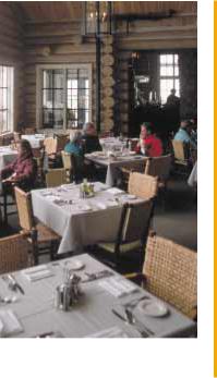
STAYING OPEN CAN BE PROFITABLE, EVEN
WITH MANY TABLES EMPTY.
CASE STUDY NEAR-EMPTY RESTAURANTS AND
OFF-SEASON MINIATURE GOLF
Have you ever walked into a restaurant for lunch and found it almost empty? Why, you might have asked, does the restaurant even bother to stay open? It might seem that the revenue from the few customers could not possibly cover the cost of running the restaurant.
In making the decision whether to open for lunch, a restaurant owner must keep in mind the distinction between fixed and variable costs. Many of a restaurant’s costs—the rent, kitchen equipment, tables, plates, silverware, and so on— are fixed. Shutting down during lunch would not reduce these costs. In other words, these costs are sunk in the short run. When the owner is deciding whether to serve lunch, only the variable costs—the price of the additional food and the wages of the extra staff—are relevant. The owner shuts down the restaurant at lunchtime only if the revenue from the few lunchtime customers fails to cover the restaurant’s variable costs.
An operator of a miniature-golf course in a summer resort community faces a similar decision. Because revenue varies substantially from season to season, the firm must decide when to open and when to close. Once again, the fixed costs—the costs of buying the land and building the course—are irrelevant. The miniature-golf course should be open for business only during those times of year when its revenue exceeds its variable costs.
THE FIRM’S LONG-RUN DECISION TO
EXIT OR ENTER A MARKET
The firm’s long-run decision to exit the market is similar to its shutdown decision. If the firm exits, it again will lose all revenue from the sale of its product, but now it saves on both fixed and variable costs of production. Thus, the firm exits the market if the revenue it would get from producing is less than its total costs.
We can again make this criterion more useful by writing it mathematically. If TR stands for total revenue, and TC stands for total cost, then the firm’s criterion can be written as
Exit if TR TC.
The firm exits if total revenue is less than total cost. By dividing both sides of this inequality by quantity Q, we can write it as
Exit if TR/Q TC/Q.
We can simplify this further by noting that TR/Q is average revenue, which equals the price P, and that TC/Q is average total cost ATC. Therefore, the firm’s exit criterion is

CHAPTER 14 FIRMS IN COMPETITIVE MARKETS |
301 |
Exit if P ATC.
That is, a firm chooses to exit if the price of the good is less than the average total cost of production.
A parallel analysis applies to an entrepreneur who is considering starting a firm. The firm will enter the market if such an action would be profitable, which occurs if the price of the good exceeds the average total cost of production. The entry criterion is
Enter if P ATC.
The criterion for entry is exactly the opposite of the criterion for exit.
We can now describe a competitive firm’s long-run profit-maximizing strategy. If the firm is in the market, it produces the quantity at which marginal cost equals the price of the good. Yet if the price is less than average total cost at that quantity, the firm chooses to exit (or not enter) the market. These results are illustrated in Figure 14-4. The competitive firm’s long-run supply curve is the portion of its marginal cost curve that lies above average total cost.
MEASURING PROFIT IN OUR GRAPH
FOR THE COMPETITIVE FIRM
As we analyze exit and entry, it is useful to be able to analyze the firm’s profit in more detail. Recall that profit equals total revenue (TR) minus total cost (TC):
Profit TR TC.
Figur e 14-4
Costs |
|
|
MC |
|
Firm’s long-run |
|
supply curve |
|
ATC |
Firm |
|
exits |
|
if |
|
P ATC |
|
0 |
Quantity |
THE COMPETITIVE FIRM’S LONG-
RUN SUPPLY CURVE. In the long run, the competitive firm’s supply curve is its marginal-cost curve (MC) above average total cost (ATC). If the price falls below average total cost, the firm is better off exiting the market.
302 |
PART FIVE FIRM BEHAVIOR AND THE ORGANIZATION OF INDUSTRY |
|
|
|
|
IN THE NEWS
Entry and Exit in
Transition Economies
Russians need only look to Poland to behold the better road untraveled. Poland too began the decade saddled with paltry living standards bequeathed by a sclerotic, centrally controlled economy run by discredited Communists. It reached out to the West for help creating monetary, budget, trade and legal regimes, and unlike Russia it followed through with sustained political will. It now ranks among Europe’s fastestgrowing economies.
Key to Poland’s steady success have been two policy decisions, and discussing them helps to illuminate by contrast what is going wrong with Russia.
competition.
The Balcerowicz rule helped break the chokehold of Communist-dominated, state-owned enterprises and Government bureaucracies over economic activity. Also, encouraging small start-ups denies organized crime opportunities for large prey.
When Poland broke away from communism, Western economists had wrung their hands trying to figure out what to do with its sprawling stateowned factories, which operated more like social welfare agencies than production units. The solution, it turned out, was benign neglect. Rather than convert factories, the Poles allowed them to
We can rewrite this definition by multiplying and dividing the right-hand side by Q:
Profit (TR/Q TC/Q) Q.
But note that TR/Q is average revenue, which is the price P, and TC/Q is average total cost ATC. Therefore,
Profit (P ATC) Q.
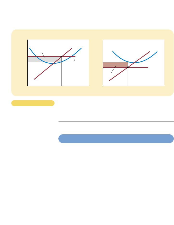
This way of expressing the firm’s profit allows us to measure profit in our graphs. Panel (a) of Figure 14-5 shows a firm earning positive profit. As we have already discussed, the firm maximizes profit by producing the quantity at which price equals marginal cost. Now look at the shaded rectangle. The height of the rectangle is P ATC, the difference between price and average total cost. The
CHAPTER 14 FIRMS IN COMPETITIVE MARKETS |
303 |
|
|
|
|
shrivel. Workers peeled away to set up retail shops and other small enterprises largely free of Government interference.
The second major decision was scarier. Poland forced insolvent firms into bankruptcy, preventing them from draining resources from productive parts of the economy. That also ended a drain on the Federal budget by firms that had to be propped up by one disguised subsidy or another.
There were moments when the post-Communist Government in Russia appeared headed in the same direction. In early 1992, the Yeltsin Government embraced the Balcerowicz rule. Russians were invited to take to the streets and set up kiosks and curbside tables, selling whatever they wanted at whatever price consumers would pay. But then Communist antibodies, in the form of the oligarchs who controlled the stateowned factories and natural resources, were activated. They detected foreign tissue and attacked. Local government buried the Balcerowicz rule, imposing licensing and other requirements and
eventually strangling start-ups. Professor Marshall Goldman of Harvard points to revealing comments by Viktor S. Chernomyrdin, the off-again, on-again Prime Minister whom President Boris N. Yeltsin restored to his post last week. Mr. Chernomyrdin observed that street vendors were an unattractive, chaotic blight on a proud country. The Russian authorities cracked down.
The impact was severe. Anders Aslund, a former adviser to the Russian Government now at the Carnegie Endowment for International Peace, estimates that since the middle of 1994, the number of enterprises in Russia has stagnated. In a typical Western economy, he estimates, there is 1 business for every 10 residents. In Russia, the ratio is 1 for every 55.
By snuffing out start-ups, Russia lost the remarkable device by which Poland drained workers out of worthless factories into units that could produce the goods that people wanted to buy.
Russia not only stifles start-ups; it also props up incompetents. It tolerates
businesses that cannot pay taxes or wages. They survive because of systems of barter and mutual forbearance of loans and taxes. Suppliers engage in round-robin lending by which everyone owes money to someone and no one ever pays up. That too throws a lifeline to insolvent firms.
Russian factories continue to churn out steel and other products that no one needs. One measure of the deformity is that Russia is littered with factories employing 10,000 or more workers. In the United States, such factories are a rarity. The effect is to keep alive concerns that chew up $1.50 worth of resources in order to turn out a product that is worth only $1 to consumers. Economists call this “negative value added.” Ordinary folk call it economic suicide.
SOURCE: The New York Times, August 30, 1998, Week in Review, p. 5.
width of the rectangle is Q, the quantity produced. Therefore, the area of the rectangle is (P ATC) Q, which is the firm’s profit.
Similarly, panel (b) of this figure shows a firm with losses (negative profit). In this case, maximizing profit means minimizing losses, a task accomplished once again by producing the quantity at which price equals marginal cost. Now consider the shaded rectangle. The height of the rectangle is ATC P, and the width is Q. The area is (ATC P) Q, which is the firm’s loss. Because a firm in this situation is not making enough revenue to cover its average total cost, the firm would choose to exit the market.
QUICK QUIZ: How does the price faced by a profit-maximizing competitive firm compare to its marginal cost? Explain. When does a profit-maximizing competitive firm decide to shut down?
304 |
PART FIVE FIRM BEHAVIOR AND THE ORGANIZATION OF INDUSTRY |
|
(a) A Firm with Profits |
(b) A Firm with Losses |
Price |
|
|
Price |
|
|
|
MC |
ATC |
|
|
|
|
Profit |
|
|
MC |
ATC |
P |
|
|
|
|
|
ATC |
P = AR = MR |
ATC |
|
|
|
|
|
P |
P = AR = MR |
|
|
|
|
Loss |
|
0 |
Q |
Quantity |
0 |
Q |
Quantity |
|
(profit-maximizing quantity) |
|
|
(loss-minimizing quantity) |
|
Figur e 14-5
PROFIT AS THE AREA BETWEEN PRICE AND AVERAGE TOTAL COST. The area of the
shaded box between price and average total cost represents the firm’s profit. The height of this box is price minus average total cost (P ATC), and the width of the box is the quantity of output (Q). In panel (a), price is above average total cost, so the firm has positive profit. In panel (b), price is less than average total cost, so the firm has losses.
THE SUPPLY CURVE IN A COMPETITIVE MARKET
Now that we have examined the supply decision of a single firm, we can discuss the supply curve for a market. There are two cases to consider. First, we examine a market with a fixed number of firms. Second, we examine a market in which the number of firms can change as old firms exit the market and new firms enter. Both cases are important, for each applies over a specific time horizon. Over short periods of time, it is often difficult for firms to enter and exit, so the assumption of a fixed number of firms is appropriate. But over long periods of time, the number of firms can adjust to changing market conditions.
THE SHORT RUN: MARKET SUPPLY WITH
A FIXED NUMBER OF FIRMS
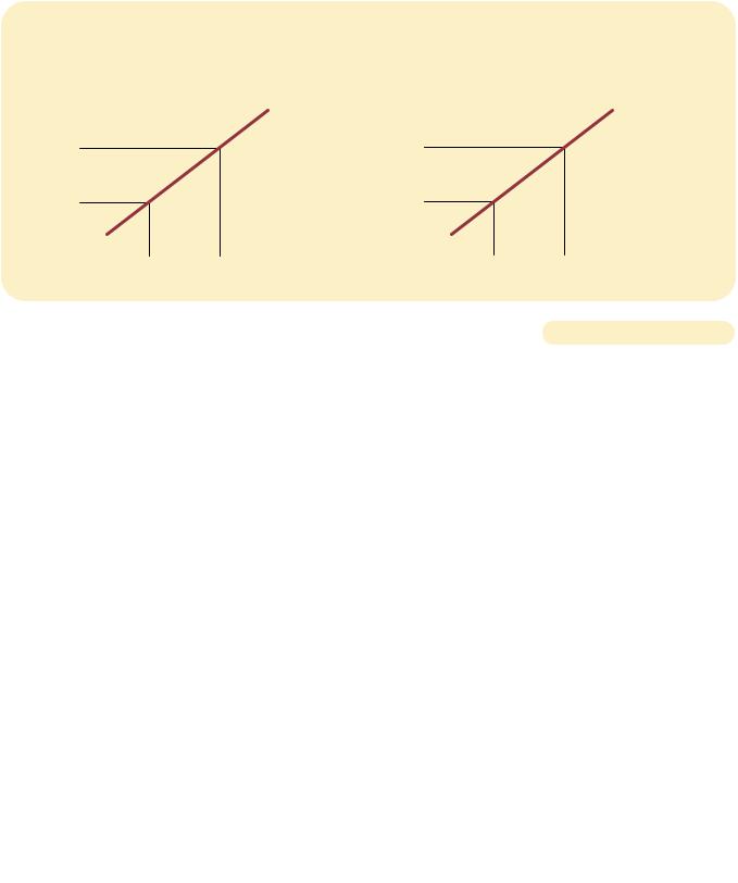
Consider first a market with 1,000 identical firms. For any given price, each firm supplies a quantity of output so that its marginal cost equals the price, as shown in panel (a) of Figure 14-6. That is, as long as price is above average variable cost, each firm’s marginal-cost curve is its supply curve. The quantity of output supplied to the market equals the sum of the quantities supplied by each of the 1,000 individual firms. Thus, to derive the market supply curve, we add the quantity supplied by each firm in the market. As panel (b) of Figure 14-6 shows, because the
|
|
|
|
|
|
CHAPTER 14 |
FIRMS IN COMPETITIVE MARKETS |
305 |
|
(a) Individual Firm Supply |
|
|
(b) Market Supply |
|
|
|
|
|
|
|
|
|
|
Price |
|
|
|
|
|
Price |
|
|
|
|
|
|
|
MC |
|
|
|
Supply |
|
|
|
|
|
|
|
|
|
|
|
$2.00 |
|
|
|
|
|
$2.00 |
|
|
|
|
|
1.00 |
|
|
|
|
|
1.00 |
|
|
|
|
|
|
|
|
|
|
|
|
|
|
|
|
|
0 |
100 |
200 |
Quantity (firm) |
0 |
|
100,000 |
200,000 Quantity (market) |
|
|
MARKET SUPPLY WITH A FIXED NUMBER OF FIRMS. When the number of firms in the |
Figur e 14-6 |
|
market is fixed, the market supply curve, shown in panel (b), reflects the individual firms’ |
|
|
|
marginal-cost curves, shown in panel (a). Here, in a market of 1,000 firms, the quantity of |
|
|
output supplied to the market is 1,000 times the quantity supplied by each firm. |
|
|
|
|
|
firms are identical, the quantity supplied to the market is 1,000 times the quantity supplied by each firm.
THE LONG RUN: MARKET SUPPLY WITH ENTRY AND EXIT
Now consider what happens if firms are able to enter or exit the market. Let’s suppose that everyone has access to the same technology for producing the good and access to the same markets to buy the inputs into production. Therefore, all firms and all potential firms have the same cost curves.
Decisions about entry and exit in a market of this type depend on the incentives facing the owners of existing firms and the entrepreneurs who could start new firms. If firms already in the market are profitable, then new firms will have an incentive to enter the market. This entry will expand the number of firms, increase the quantity of the good supplied, and drive down prices and profits. Conversely, if firms in the market are making losses, then some existing firms will exit the market. Their exit will reduce the number of firms, decrease the quantity of the good supplied, and drive up prices and profits. At the end of this process of entry and exit, firms that remain in the market must be making zero economic profit. Recall that we can write a firm’s profits as
Profit (P ATC) Q.
This equation shows that an operating firm has zero profit if and only if the price of the good equals the average total cost of producing that good. If price is above average total cost, profit is positive, which encourages new firms to enter. If price
306 |
PART FIVE FIRM BEHAVIOR AND THE ORGANIZATION OF INDUSTRY |
is less than average total cost, profit is negative, which encourages some firms to exit. The process of entry and exit ends only when price and average total cost are driven to equality.
This analysis has a surprising implication. We noted earlier in the chapter that competitive firms produce so that price equals marginal cost. We just noted that free entry and exit forces price to equal average total cost. But if price is to equal both marginal cost and average total cost, these two measures of cost must equal each other. Marginal cost and average total cost are equal, however, only when the firm is operating at the minimum of average total cost. Therefore, the long-run equilibrium of a competitive market with free entry and exit must have firms operating at their efficient scale.
Panel (a) of Figure 14-7 shows a firm in such a long-run equilibrium. In this figure, price P equals marginal cost MC, so the firm is profit-maximizing. Price also equals average total cost ATC, so profits are zero. New firms have no incentive to enter the market, and existing firms have no incentive to leave the market.
From this analysis of firm behavior, we can determine the long-run supply curve for the market. In a market with free entry and exit, there is only one price consistent with zero profit—the minimum of average total cost. As a result, the long-run market supply curve must be horizontal at this price, as in panel (b) of Figure 14-7. Any price above this level would generate profit, leading to entry and an increase in the total quantity supplied. Any price below this level would generate losses, leading to exit and a decrease in the total quantity supplied. Eventually, the number of firms in the market adjusts so that price equals the minimum of
(a) Firm’s Zero-Profit Condition |
(b) Market Supply |
Price |
Price |
MC
ATC
P = minimum 
 Supply
ATC
0 Quantity (firm) 0 Quantity (market)
Figur e 14-7
MARKET SUPPLY WITH ENTRY AND EXIT. Firms will enter or exit the market until profit is driven to zero. Thus, in the long run, price equals the minimum of average total cost,
as shown in panel (a). The number of firms adjusts to ensure that all demand is satisfied at this price. The long-run market supply curve is horizontal at this price, as shown in panel (b).
CHAPTER 14 FIRMS IN COMPETITIVE MARKETS |
307 |
average total cost, and there are enough firms to satisfy all the demand at this price.
WHY DO COMPETITIVE FIRMS STAY IN BUSINESS
IF THEY MAKE ZERO PROFIT?
At first, it might seem odd that competitive firms earn zero profit in the long run. After all, people start businesses to make a profit. If entry eventually drives profit to zero, there might seem to be little reason to stay in business.
To understand the zero-profit condition more fully, recall that profit equals total revenue minus total cost, and that total cost includes all the opportunity costs of the firm. In particular, total cost includes the opportunity cost of the time and money that the firm owners devote to the business. In the zero-profit equilibrium, the firm’s revenue must compensate the owners for the time and money that they expend to keep their business going.
Consider an example. Suppose that a farmer had to invest $1 million to open his farm, which otherwise he could have deposited in a bank to earn $50,000 a year in interest. In addition, he had to give up another job that would have paid him $30,000 a year. Then the farmer’s opportunity cost of farming includes both the interest he could have earned and the forgone wages—a total of $80,000. Even if his profit is driven to zero, his revenue from farming compensates him for these opportunity costs.
Keep in mind that accountants and economists measure costs differently. As we discussed in Chapter 13, accountants keep track of explicit costs but usually miss implicit costs. That is, they measure costs that require an outflow of money from the firm, but they fail to include opportunity costs of production that do not involve an outflow of money. As a result, in the zero-profit equilibrium, economic profit is zero, but accounting profit is positive. Our farmer’s accountant, for instance, would conclude that the farmer earned an accounting profit of $80,000, which is enough to keep the farmer in business.
“We’re a nonprofit organization—we don’t intend to be, but we are!”