292 |
PART FIVE FIRM BEHAVIOR AND THE ORGANIZATION OF INDUSTRY |
is small compared to the size of the market and, therefore, has little ability to influence market prices. By contrast, if a firm can influence the market price of the good it sells, it is said to have market power. In the three chapters that follow this one, we examine the behavior of firms with market power, such as your local water company.
Our analysis of competitive firms in this chapter will shed light on the decisions that lie behind the supply curve in a competitive market. Not surprisingly, we will find that a market supply curve is tightly linked to firms’ costs of production. (Indeed, this general insight should be familiar to you from our analysis in Chapter 7.) But among a firm’s various costs—fixed, variable, average, and mar- ginal—which ones are most relevant for its decision about the quantity to supply? We will see that all these measures of cost play important and interrelated roles.
WHAT IS A COMPETITIVE MARKET?
competitive market
a market with many buyers and sellers trading identical products so that each buyer and seller is a price taker
Our goal in this chapter is to examine how firms make production decisions in competitive markets. As a background for this analysis, we begin by considering what a competitive market is.
THE MEANING OF COMPETITION
Although we have already discussed the meaning of competition in Chapter 4, let’s review the lesson briefly. A competitive market, sometimes called a perfectly competitive market, has two characteristics:
There are many buyers and many sellers in the market.
The goods offered by the various sellers are largely the same.
As a result of these conditions, the actions of any single buyer or seller in the market have a negligible impact on the market price. Each buyer and seller takes the market price as given.
An example is the market for milk. No single buyer of milk can influence the price of milk because each buyer purchases a small amount relative to the size of the market. Similarly, each seller of milk has limited control over the price because many other sellers are offering milk that is essentially identical. Because each seller can sell all he wants at the going price, he has little reason to charge less, and if he charges more, buyers will go elsewhere. Buyers and sellers in competitive markets must accept the price the market determines and, therefore, are said to be price takers.
In addition to the foregoing two conditions for competition, there is a third condition sometimes thought to characterize perfectly competitive markets:
Firms can freely enter or exit the market.

294 |
PART FIVE FIRM BEHAVIOR AND THE ORGANIZATION OF INDUSTRY |
|
|
How much revenue does the farm receive for the typical gallon of milk? |
|
|
How much additional revenue does the farm receive if it increases |
|
|
|
production of milk by 1 gallon? |
|
|
The last two columns in Table 14-1 answer these questions. |
average r evenue |
|
The fourth column in the table shows average revenue, which is total revenue |
total revenue divided by the quantity |
(from the third column) divided by the amount of output (from the first column). |
sold |
|
Average revenue tells us how much revenue a firm receives for the typical unit |
|
|
sold. In Table 14-1, you can see that average revenue equals $6, the price of a gal- |
|
|
lon of milk. This illustrates a general lesson that applies not only to competitive |
|
|
firms but to other firms as well. Total revenue is the price times the quantity |
|
|
(P Q), and average revenue is total revenue (P Q) divided by the quantity (Q). |
|
|
Therefore, for all firms, average revenue equals the price of the good. |
mar ginal r evenue |
|
The fifth column shows marginal revenue, which is the change in total rev- |
the change in total revenue from an |
enue from the sale of each additional unit of output. In Table 14-1, marginal rev- |
additional unit sold |
enue equals $6, the price of a gallon of milk. This result illustrates a lesson that |
|
|
applies only to competitive firms. Total revenue is P Q, and P is fixed for a com- |
|
|
petitive firm. Therefore, when Q rises by 1 unit, total revenue rises by P dollars. For |
|
|
competitive firms, marginal revenue equals the price of the good. |
|
|
|
QUICK QUIZ: When a competitive firm doubles the amount it sells, what |
|
|
|
|
|
|
happens to the price of its output and its total revenue? |
|
|
|
PROFIT MAXIMIZATION AND THE
COMPETITIVE FIRM’S SUPPLY CURVE
The goal of a competitive firm is to maximize profit, which equals total revenue minus total cost. We have just discussed the firm’s revenue, and in the last chapter we discussed the firm’s costs. We are now ready to examine how the firm maximizes profit and how that decision leads to its supply curve.
A SIMPLE EXAMPLE OF PROFIT MAXIMIZATION
Let’s begin our analysis of the firm’s supply decision with the example in Table 14-2. In the first column of the table is the number of gallons of milk the Smith Family Dairy Farm produces. The second column shows the farm’s total revenue, which is $6 times the number of gallons. The third column shows the farm’s total cost. Total cost includes fixed costs, which are $3 in this example, and variable costs, which depend on the quantity produced.
The fourth column shows the farm’s profit, which is computed by subtracting total cost from total revenue. If the farm produces nothing, it has a loss of $3. If it produces 1 gallon, it has a profit of $1. If it produces 2 gallons, it has a profit of $4, and so on. To maximize profit, the Smith Farm chooses the quantity that makes profit as large as possible. In this example, profit is maximized when the farm produces 4 or 5 gallons of milk, when the profit is $7.
CHAPTER 14 FIRMS IN COMPETITIVE MARKETS |
295 |
|
QUANTITY |
TOTAL |
|
|
MARGINAL |
MARGINAL |
|
(IN GALLONS) |
REVENUE |
TOTAL COST |
PROFIT |
REVENUE |
COST |
|
|
|
|
|
|
|
|
(Q) |
(TR) |
(TC) |
(TR TC) |
(MR ∆TR/∆Q) |
(MC ∆TC/∆Q) |
|
|
|
|
|
|
|
|
0 |
$ 0 |
$ 3 |
$3 |
$6 |
$2 |
|
1 |
6 |
5 |
1 |
|
6 |
3 |
|
2 |
12 |
8 |
4 |
|
6 |
4 |
|
3 |
18 |
12 |
6 |
|
6 |
5 |
|
4 |
24 |
17 |
7 |
|
6 |
6 |
|
5 |
30 |
23 |
7 |
|
6 |
7 |
|
6 |
36 |
30 |
6 |
|
6 |
8 |
|
7 |
42 |
38 |
4 |
|
6 |
9 |
|
8 |
48 |
47 |
1 |
|
|
|
PROFIT MAXIMIZATION: A NUMERICAL EXAMPLE
Table 14-2
There is another way to look at the Smith Farm’s decision: The Smiths can find the profit-maximizing quantity by comparing the marginal revenue and marginal cost from each unit produced. The last two columns in Table 14-2 compute marginal revenue and marginal cost from the changes in total revenue and total cost. The first gallon of milk the farm produces has a marginal revenue of $6 and a marginal cost of $2; hence, producing that gallon increases profit by $4 (from $3 to $1). The second gallon produced has a marginal revenue of $6 and a marginal cost of $3, so that gallon increases profit by $3 (from $1 to $4). As long as marginal revenue exceeds marginal cost, increasing the quantity produced raises profit. Once the Smith Farm has reached 5 gallons of milk, however, the situation is very different. The sixth gallon would have marginal revenue of $6 and marginal cost of $7, so producing it would reduce profit by $1 (from $7 to $6). As a result, the Smiths would not produce beyond 5 gallons.
One of the Ten Principles of Economics in Chapter 1 is that rational people think at the margin. We now see how the Smith Family Dairy Farm can apply this principle. If marginal revenue is greater than marginal cost—as it is at 1, 2, or 3 gal- lons—the Smiths should increase the production of milk. If marginal revenue is less than marginal cost—as it is at 6, 7, or 8 gallons—the Smiths should decrease production. If the Smiths think at the margin and make incremental adjustments to the level of production, they are naturally led to produce the profit-maximizing quantity.
THE MARGINAL-COST CURVE AND THE
FIRM’S SUPPLY DECISION
To extend this analysis of profit maximization, consider the cost curves in Figure 14-1. These cost curves have the three features that, as we discussed in Chapter 13, are thought to describe most firms: The marginal-cost curve (MC) is upward sloping. The average-total-cost curve (ATC) is U-shaped. And the marginal-cost curve
296 |
PART FIVE FIRM BEHAVIOR AND THE ORGANIZATION OF INDUSTRY |
Figur e 14-1
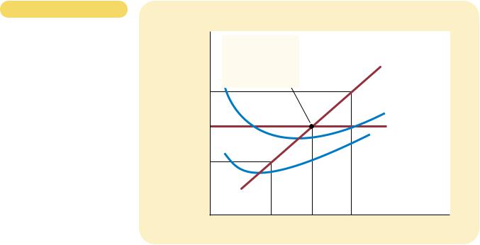
PROFIT MAXIMIZATION FOR A
COMPETITIVE FIRM. This figure shows the marginal-cost curve (MC), the average-total-cost curve (ATC), and the average- variable-cost curve (AVC). It also shows the market price (P), which equals marginal revenue (MR) and average revenue (AR). At the quantity Q1, marginal revenue MR1 exceeds marginal cost MC1, so raising production increases profit. At the quantity Q2, marginal cost MC2 is above marginal revenue MR2, so reducing production increases profit. The profit-maximizing quantity QMAX is found where the horizontal price line intersects the marginal-cost curve.
Costs
and
Revenue
MC2
P = MR1 = MR2
MC1
0
The firm maximizes profit by producing the quantity at which marginal cost equals marginal revenue.
crosses the average-total-cost curve at the minimum of average total cost. The figure also shows a horizontal line at the market price (P). The price line is horizontal because the firm is a price taker: The price of the firm’s output is the same regardless of the quantity that the firm decides to produce. Keep in mind that, for a competitive firm, the firm’s price equals both its average revenue (AR) and its marginal revenue (MR).
We can use Figure 14-1 to find the quantity of output that maximizes profit. Imagine that the firm is producing at Q1. At this level of output, marginal revenue is greater than marginal cost. That is, if the firm raised its level of production and sales by 1 unit, the additional revenue (MR1) would exceed the additional costs (MC1). Profit, which equals total revenue minus total cost, would increase. Hence, if marginal revenue is greater than marginal cost, as it is at Q1, the firm can increase profit by increasing production.
A similar argument applies when output is at Q2. In this case, marginal cost is greater than marginal revenue. If the firm reduced production by 1 unit, the costs saved (MC2) would exceed the revenue lost (MR2). Therefore, if marginal revenue is less than marginal cost, as it is at Q2, the firm can increase profit by reducing production.
Where do these marginal adjustments to level of production end? Regardless of whether the firm begins with production at a low level (such as Q1) or at a high level (such as Q2), the firm will eventually adjust production until the quantity produced reaches QMAX. This analysis shows a general rule for profit maximization: At the profit-maximizing level of output, marginal revenue and marginal cost are exactly equal.
We can now see how the competitive firm decides the quantity of its good to supply to the market. Because a competitive firm is a price taker, its marginal
CHAPTER 14 FIRMS IN COMPETITIVE MARKETS |
297 |
Price |
|
|
|
|
|
|
MC |
P2 |
|
|
|
|
|
|
ATC |
P1 |
|
|
|
|
|
|
AVC |
0 |
Q1 |
Q2 |
Quantity |
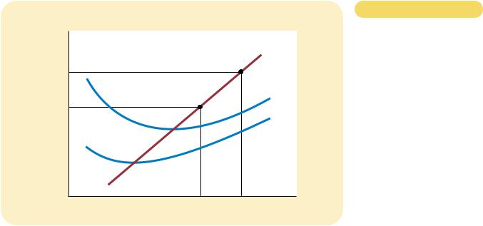
Figur e 14-2
MARGINAL COST AS THE
COMPETITIVE FIRM’S SUPPLY
CURVE. An increase in the price from P1 to P2 leads to an increase in the firm’s profit-maximizing quantity from Q1 to Q2. Because the marginal-cost curve shows the quantity supplied by the firm at any given price, it is the firm’s supply curve.
revenue equals the market price. For any given price, the competitive firm’s profitmaximizing quantity of output is found by looking at the intersection of the price with the marginal-cost curve. In Figure 14-1, that quantity of output is QMAX.
Figure 14-2 shows how a competitive firm responds to an increase in the price. When the price is P1, the firm produces quantity Q1, which is the quantity that equates marginal cost to the price. When the price rises to P2, the firm finds that marginal revenue is now higher than marginal cost at the previous level of output, so the firm increases production. The new profit-maximizing quantity is Q2, at which marginal cost equals the new higher price. In essence, because the firm’s marginal-cost curve determines the quantity of the good the firm is willing to supply at any price, it is the competitive firm’s supply curve.
THE FIRM’S SHORT-RUN DECISION TO SHUT DOWN
So far we have been analyzing the question of how much a competitive firm will produce. In some circumstances, however, the firm will decide to shut down and not produce anything at all.
Here we should distinguish between a temporary shutdown of a firm and the permanent exit of a firm from the market. A shutdown refers to a short-run decision not to produce anything during a specific period of time because of current market conditions. Exit refers to a long-run decision to leave the market. The short-run and long-run decisions differ because most firms cannot avoid their fixed costs in the short run but can do so in the long run. That is, a firm that shuts down temporarily still has to pay its fixed costs, whereas a firm that exits the market saves both its fixed and its variable costs.
For example, consider the production decision that a farmer faces. The cost of the land is one of the farmer’s fixed costs. If the farmer decides not to produce any