9Image Quality and Artifacts

Добавил:

Upload Опубликованный материал нарушает ваши авторские права? Сообщите нам.

Вуз:

Томский Политехнический Университет

Предмет:

[НЕСОРТИРОВАННОЕ]

Файл:

Buzug_Computed_tomography_From_photon_stat.pdf

Скачиваний:

Добавлен:

29.05.2015

Размер:

15.29 Mб

Скачать

☆

<<< < Предыдущая 1 2 3 45 / 75 6 7 > Следующая >>>

9.2 Modulation Transfer Function of the Imaging Process

With the impulse response

Contents
9.1	Introduction . . . . . . . . . . . . . . . . . . . . . . . . . . . . . . . . . . . . . . . . . . . . . . . . . . . . . . .	403
9.2	Modulation Transfer Function of the Imaging Process . . . . . . . . . . . . . . . . . . . . . . . . .	404
9.3	Modulation Transfer Function and Point Spread Function . . . . . . . . . . . . . . . . . . . . . .	410
9.4	Modulation Transfer Function in Computed Tomography . . . . . . . . . . . . . . . . . . . . . .	412
9.5	SNR, DQE, and ROC . . . . . . . . . . . . . . . . . . . . . . . . . . . . . . . . . . . . . . . . . . . . . . . . .	421
9.6	D Artifacts . . . . . . . . . . . . . . . . . . . . . . . . . . . . . . . . . . . . . . . . . . . . . . . . . . . . . . . .	423
9.7	D Artifacts . . . . . . . . . . . . . . . . . . . . . . . . . . . . . . . . . . . . . . . . . . . . . . . . . . . . . . . .	445
9.8	Noise in Reconstructed Images . . . . . . . . . . . . . . . . . . . . . . . . . . . . . . . . . . . . . . . . . .	462

9.1 Introduction

The physical attenuation values f (x, y) of the human tissue within an axial slice are distributed continuously in value and space. In the previous chapter it has become evident that in practice it is indispensable for computed tomography (CT) to digitize the acquired data in order to carry out the mathematical object reconstruction. This means that the attenuation of the radiation must be measured, digitalized, and stored. Within this processing chain, the continuous physical signal is discretized in the spatial domain and the values have to be quantized. Figure . shows that this process can be modeled as a signal transmission chain. One can thus evaluate the changes – in general the deterioration – to which the signal f (x, y) is subjected during acquisition and discretization into a series of numbers g(n, m) and further on until the tomogram c(n, m) is displayed and presented to the clinician.

The signal path is to be modeled with ﬁve layers. The ﬁrst layer, which is called the physical layer or X-ray imaging layer, describes the beam characteristic . T his layer must be considered analogously to the lens system of a camera because the physical quality of the X-ray optical system is described by the focus spot size in

The physical parameters inﬂuencing the image quality can of course be evaluated retro-

spectively only, i.e., after the image has been reconstructed. This is due to the fact that an image f (x, y) is not available at the focal spot of the X-ray tube.

9 Image Quality and Artifacts

the X-ray tube and by the slice collimation of the X-ray fan. The transfer functions (H and H ) describe the change of the spatially continuous and value-continuous input signal f (x, y). The physical nature of the signal initially remains unchanged. However, the interaction between the imaging radiation and the object generally also changes the physical nature of the radiation regarding hardening of the spectrum of polychromatic X-ray. This may be compared with the chromatic aberration of a camera lens system. The image, which has been degenerated by beam hardening (H ), is denoted by b(x, y).

The sensor or detector layer (analogous to the ﬁlm plane of a conventional optical camera) is the second layer. Here, the signal is subdivided by an anti-scatter grid beam collimation (H ) and then physically transformed. That is, the X-ray photons are, for example, detected with a scintillation crystal and then converted into an electrical signal e(x, y) with an attached photomultiplier or photodiode. Here, among others, crystal properties such as afterglow (H ) have to be modeled.

In practice, spatial discretization will already occur in the sensor or detector layer. However, for a better separation of each cause of signal deterioration, this effect is modeled in the third layer – the electronic or digitalization layer – in which the electrical signal of the photomultiplier or the photodiode (cf. Fig. . ) is spatially discretized (H ). Furthermore, the values are quantized (H ) by an acquisition with an analog–digital converter (ADC).

In the fourth layer – the reconstruction or algorithm layer – the size of the image matrix to be reconstructed together with the corresponding detector interpolation (H ) as well as the special properties of the ﬁlter kernels used for the ﬁltered backprojection (H ) are modeled.

The last layer – the image processing and display layer – models the type of image representation. An example is, for instance, the mapping of the physical attenuation values onto a gray-value interval (H ), which is appropriate for human perception as well as the quality of the visualization medium, for example, the monitor (H ).

In the following sections of this chapter, it will be shown how the individual factors of the imaging chain that inﬂuence each part can be quantiﬁed. In this context, the so-called modulation transfer function (MTF) plays an important role.

9.2

Modulation Transfer Function of the Imaging Process

With the transfer functions H through H in the chart shown in Fig. . , the imaging, or more precisely, the alteration of the representation of an object f (x, y) can be described mathematically (cf. Sect. . ). These functions are generally available as amplitude and phase curves as a function of the spatial frequency, i.e., as H(u, v). From a technical point of view, it is interesting how the spatial resolution is changed by each individual element of the system chain during the imaging process. The commonly used unit of the spatial resolution is [lp/mm], i.e., line pairs per

9.2 Modulation Transfer Function of the Imaging Process

Fig. . . The image acquisition process can be modeled in signal transmission layers from the X-ray tube to the visualization of the image data on a display

millimeter . The spatial resolution thus indicates how close two neighboring lines can get to each other before they can no longer be distinguished due to the vanishing modulation of the image values, i.e., the variation of the gray values between the lines. An important parameter related to the evaluation of the spatial resolution is the contrast

max

(

x, y

) +

min

(

x, y

)

max

(x, y) − min

(x, y)

( . )

of the image, i.e., the variation interval of the image values around the mean value, normalized by the mean value.

This is because resolution cannot be deﬁned by the visibility of a small single object. It is rather deﬁned by the ability to su ciently separate two neighboring objects.

The contrast is also called modulation.

9 Image Quality and Artifacts

In this section it will be explained why the modulation transfer function is a suitable measure for the spatial resolution. One should initially assume that Fig. . shows a one-dimensional sinusoidal gray-value distribution

f (x) = + C sin( πux)

( . )

of an image. It is further assumed that the parameter u is again the spatial frequency.

Fig. . . Motivation of the modulation transfer function (MTF). Top: A sinusoidal signal is blurred by a Gaussian impulse response. Center: Transfer of a narrow strip with a width of ξ via f (ξ)h(x − ξ) ξ. Bottom: The entire image results from the convolution of the original signal with the impulse response f (x) h(x)

which causes a Gaussian blurring, the following mapping of a narrow image strip ξ at the point ξ can be found


b (x) = f (ξ)h(x − ξ)	ξ =	6		f (ξ)e−(x−ξ)	ξ .	( . )
			π

( . ) represents the blurring caused by the imaging or transfer system. The entire image obviously results from the convolution b(x) = f (x) > h(x) of the original signal f (x) with the impulse response h(x), i.e., from

(

)

(

−

)

= 6π

(

)

) =−

−

∫

dξ

∫

e−(x−ξ) dξ .

Since the convolution is symmetric, one may also write

(

−

)

(

)

= 6π

(

−

)

) =−

−

∫

dξ

∫

e−ξ dξ .

If the gray-value distribution ( . ) is substituted into ( . ), one ﬁnds

b(x) = ∫ ( + C sin( πu(x − ξ))) h(ξ)dξ .

−

Taking into account the addition law for the sine

sin(α − β) = sin(α)cos(β) − cos(α)sin(β) ,

( . ) can be converted into


b(x) = ∫ h(ξ)dξ +	∫ C sin( πux)cos( πuξ)h(ξ)dξ + . . .

− −

. . . − ∫ C cos( πux)sin( πuξ)h(ξ)dξ

−

=∫ h(ξ)dξ + C sin( πux) ∫ cos( πuξ)h(ξ)dξ + . . .

−

. . . − C cos( πux) ∫ sin( πuξ)h(ξ)dξ .

( . )

−

9 Image Quality and Artifacts

As the two last integral terms in ( . ) look like components of a vector, the expression

cos

πux h x dx

∫

sin

πux h x dx

( . )

n ∫

(

) ( )

(

) ( )

= on

−

may be interpreted as the length of a vector. From this point of view, the phase can be expressed via

cos(φ) =

−∫

cos( πux)h(x)dx

( . )

or by

sin(φ) =

−∫

sin( πux)h(x)dx .

( . )

Since the impulse response is normalized to , i.e.,

(

)

−

∫ h

( . )

the image can be expressed as

b x

εC sin πux

cos

) −

εC cos

πux

)

sin

(

)

( . )

or, again using( the) =addition+

law( ( . ),)as

(

b(x) = + εC sin( πux − φ) .

( . )

( . ) is thus the mapping of the object, represented by ( . ), via the transfer system. To be able to interpret the value ε, one still has to verify that ε always ranges between and . This is directly due to the normalization ( . ) of the impulse re-

sponse, since

(

)

(

)

(

)

=−

−

e−i πux dx

∫

(

)

(

)

−

) (

)

−

(

( . )

∫

cos πux

∫

sin πux

(

)

(

)

(

)

(

−

cos

πux

−

sin

πux

)

ε .

∫

dx!

∫ h

dx!

9.2 Modulation Transfer Function of the Imaging Process

Thus, ε may be interpreted as the MTF, since this variable obviously controls the modulation of the image during the transfer through a system with the impulse response h(x).

Again, looking at ( . ) reveals that ε depends on the spatial frequency such that one may write

	=	(	) =		(		)		H
	=	(	) =	H−	(		)		H
ε		MTF u		∫	h	x		e−i πux dx		,	( . )

where the normalization MTF( ) = shall apply.

The relation with the contrast function ( . ) can now be interpreted as follows. The object contrast – for simplicity described for the one-dimensional case – is deﬁned as

C = max

f (x) − min

f (x) .

max

min

In analogy, the contrast of the

mapped pattern is deﬁned as

( ) +

(

)

Cb = εC = max

b(x) − min

b(x) .

max

b x

min

b x

This means that the MTF

(

)

reads

(

) +

( )

ε = MTF(u) = Cb C

max b(x) − min b(x)

=max b(x) + min b(x)

max f (x) − min f (x) max f (x) + min f (x)

( . )

and is thus the frequency-dependent ratio of the image contrast to the object contrast. Figure . shows a typical proﬁle of the MTF. The proﬁle must be interpreted such that the constant component of the image, i.e., MTF( ), is always perfectly

Fig. . . Proﬁle of the frequency-dependent MTF(u). Steeply decreasing curves characterize poor image transmission quality (dashed curve)

9 Image Quality and Artifacts

transmitted. With increasing spatial frequency of the structures in the object to be imaged, the contrast in the image decreases. The faster the MTF decreases, the poorer the quality of the transmitted image becomes.

The complete MTF of a system consisting of several components in the imaging chain is the product of the corresponding MTFs of the individual components. Regarding Fig. . , this means, for example,

MTFsystem(u) = MTFX-ray layer(u) ċ MTFdetector layer(u) ċ MTFelectronics layer(u) ċ . . .

. . . ċ MTFalgorithm layer(u) ċ MTFdisplay layer(u)

( . )

with

MTFX-ray layer	u	MTFX-ray source			u	MTFcollimator				u . . .
		. . .	ċ	MTF			(	u	)		( . )
					matter interaction
(	) =								(	) ċ
				photon-( ) ċ

and further layers in analogy to the above equations. ( . ) indicates that the weakest transfer element in the chain dominates the MTF of the entire system and thus the imaging quality.

9.3

Modulation Transfer Function and Point Spread Function

The MTF can be easily set in relation to the Fourier transform of the point spread function (PSF). Therefore, one has to assume that a δ spike is located in the Cartesian x–y image plane. As shown in Sect. . , the imaging system generates a special image g(x, y) of that point – the point image. With a δ spike as an input signal, i.e. a point being the object to be imaged, the resulting image is actually identical to the PSF of the imaging system.

Taking into account the conditions of linearity and shift invariance of the imaging system one can use the Fourier transform to ﬁnd the expression

(			(		)
(	) =− −		(		)
OTF u, v	∫ ∫	h		x, y		e− πi(xu+yv)dx dy ,	( . )

called the optical transfer function (OTF) (Lehmann et al. ). The absolute value of the optical transfer function is then the MTF

MTF(u, v) = OTF(u, v) . ( . )

In general, the OTF is a complex expression so that it can be divided into the absolute value and phase

OTF(u, v) = MTF(u, v)eiPT F(u,v) .

( . )

9.3 Modulation Transfer Function and Point Spread Function

The PTF is called the phase transfer function. In summary, ( . ) may thus be described by


PSF ——— OTF		u, v	) =		MTF	u, v	)	eiPT F(u,v)
If the radial frequencyAis deﬁned•	as(		) =		(		)		.	( . )
	q = 6									( . )
	q = 6			u + v						( . )

and if it is initially assumed that v = , to use the example described in the previous section, ( . ) reads

(

)

OTF

∫

∫ h

x, y

e− πix q dx dy

) =− −

( . )

(

)

=−

−

∫

x, y

dy! e− πix q dx .

The bracketed expression is the line spread function L(x). One therefore writes

(

) =

(

) =

(

)

H−

MTF

OTF q,

∫

e− πix q dx

( . )

According to Krestel ( ) the MTF is thus the absolute value of the one-dimen- sional Fourier transform of the line spread function. In the one-dimensional example, described in the previous section, the line spread function can be identiﬁed by the PSF. For this purpose, one may compare the ( . ) with ( . ).

In practice, it may happen that the phase changes during the signal transfer through the system. If, for example, the image grid b(x) is shifted by π with respect to the object grid g(x), then a wave trough of b(x) just falls onto a wave crest of g(x). In doing so, dark structures will be displayed bright and bright structures dark. This e ect is called pseudo-sharpness. Figure . illustrates this e ect on the MTF. In the frequency range q < q < q , the image is reproduced with inverted phases (Morneburg ).

Fig. . . Proﬁle of the frequency-dependent MTF(u) with pseudo-sharpness

9 Image Quality and Artifacts

9.4

Modulation Transfer Function in Computed Tomography

For quantitative and thus objective evaluation of the imaging quality in CT, the concept of the MTF has indeed proved to be useful. The corresponding approach is described by means of ( . ), where the system is decomposed into its components. The ﬁrst step consists of separating the technical image generation process from the image reconstruction algorithm, thus

MTFC T	q		MTFimaging hardware	q		MTF imaging software q		.	( . )
represents layers through of Fig. . and the second factor layer .
The ﬁrst factor (		) =	(		) ċ	(	)

Layer will be not be dealt with here.

Concerning the hardware part that is related to the image generation process, two components, namely the X-ray source and the detector, play a particularly important role. In the following, the focal spot size of the X-ray tube and the spatial discretization of the detector array will be discussed in detail. These two issues are represented in Fig. . by H in layer and by H in layer . As suggested by ( . ), one may also consider these two components separately and then multiply the individual MTFs of the components, i.e.,

MTFimaging hardware(q) = MTFX-ray source(q) ċ MTFsampling(q) . ( . )

Starting with the X-ray source, the size of the target point of the electrons on the anode has to be interpreted as the spatial dimension of the X-ray source. In fact, the size of the focal spot on the rotating anode depends on several parameters, such as on the angle under which the detector “sees” the spot. Furthermore, the tube power plays an important role, too. Typical focal spots in clinical applications have a diameter of approximately mm (cf. Sect. . . ).

Figure . shows the situation for an X-ray source with a focus diameter F. T he detector, which has a distance FDD from the source, is initially assumed to be ideally punctiform because one actually considers the components separately. Therefore, the detector does not contribute to image deterioration in this ﬁrst step.

A point located in the center of the measurement ﬁeld (the distance between the focus and the center will be denoted the focus center distance, FCD, and the focus detector distance, FDD, will be assumed to be FCD) generates on the punctiform detector – according to the intercept theorem – an inverse rectangular function of the length

	=		−		=
bF		F FDD		FCD		F .	( . )
		FDD

This rectangular signal is the PSF, i.e., the impulse response of the imaging system, since it is in fact the image of a δ object in the center of the measurement ﬁeld. If

Iξ (ξ) = I − b˜F rect bF				( . )
			ξ

			9.4 Modulation Transfer Function in Computed Tomography

Fig. . . Deconstruction of the imaging system into its components to determine the individual MTFs for each element. Illustration of a real X-ray source with a focal spot diameter F and an ideal punctiform detector

is the inverse rectangle with a length bF – where bF is a dimensionless normalization length bF ( m) – then the modulation transfer function may be easily determined on the basis of the Fourier transform of the impulse response, i.e., by

MTFX-ray source(q) = 9sin(πbF q)9 ( . )

πbF q

(cf. Sect. . ).

If the detector is considered a second component of the imaging chain, then one readily sees that a ﬁnite aperture must always be taken into account for real systems. In analogy to the ﬁrst step, one also starts here by idealizing all the other components. The focus of the X-ray source will thus be assumed to have a zero diameter in this second step.

The object is scanned with a rectangular sensitivity proﬁle here, i.e. the detector is integrated over its length ξ. For a δ object in the center of the measurement ﬁeld this means that a signal is acquired, which – similar to ( . ) and also according to the intercept theorem – has the length

bD =		FCD	=	ξ
	ξ				.	( . )
		FDD

Figure . readily illustrates this fact. This sensitivity proﬁle represents the required impulse response

Ij(ξ) = I − b˜D rect bD .				( . )
			ξ

	9 Image Quality and Artifacts

Fig. . . Deconstruction of the imaging system into its components to determine the individual MTFs. Illustration of an ideal punctiform X-ray source and a real detector consisting of elements of size ξ

The MTF can again be determined by means of the Fourier transform from this

inverse rectangle with a length bD (where bD is the dimensionless normalization length bD ( m)). The result reads

	(		) = 9	sin	(	D		)9
MTFsampling		q		πb			q		.	( . )
				πb			q

For the major hardware parts of the imaging system chain one now ﬁnds the MTF

MTFimaging hardware

(

) =

sin πbF

(

) ċ

(

)

MTFX-ray source

MTFsampling

= 9

( F

)99

(

( . )

sin

πb

πb q

πb

Figure . shows the behavior of the total MTF. Indeed it is obvious that the weakest component of the imaging system chain impairs the ﬁnal result. The ﬁrst root of the MTF is called the cut-o frequency. T his is the maximum frequency of spatial structures that can be resolved by the system.

The magnitudes of the cut-o frequencies given in Fig. . are simply estimated values that have to be adapted to the corresponding real situation. Depending on the design of the tube, which is frequently designed as a ﬂying focal spot system, the terms in ( . ) must be computed accordingly.

In order to provide another example for the assessment of the image quality, the MTF of the reconstruction algorithm will be estimated according to ( . ). Regarding the ﬁltered backprojection, the MTF shown in layer of Fig. . consists of the

	9.4 Modulation Transfer Function in Computed Tomography

Fig. . . MTFs for the X-ray source, for the sampling process with a ﬁnite detector aperture, and for the major hardware parts of the imaging system chain (from top to bottom)

following components

MTFalgorithm(q) = MTFinterpolation(q) ċ MTFfilter kernel(q) . ( . )

9 Image Quality and Artifacts

The ﬁrst term in ( . ) describes the image transfer behavior through interpolation.

The projection values must be interpolated because the projection proﬁle is scanned

with detector elements with a width

ξ. As already described in

Sect. . . , the

required point of the image mask is usually not available on an exact sampling point

of the projection or the ﬁltered projection. Figure . illustrates this problem with

a very coarse sampling grid, ξ, of the ﬁltered projection.

In order to illustrate the MTF for the interpolation process, one has to discuss

the interpolation itself. If a required value is not found on the grid of the available

values, then this value must be interpolated from the neighboring points.

This, formally, is the convolution

hγ (ξ ) = hγ (j ξ)l(ξ − j ξ) .

( . )

In this context, the ideal convolution kernel l

results from the sampling theo-

a periodic spectrum, an appropriate

rem (cf. Sect. . ). As sampled signals have ( )

has to be chosen within the inverse Fourier transform when the signal is

window

reconstructed from the spectrum. Under ideal conditions, a multiplication of the

spectrum with a rectangular window is used for this purpose. In the spatial domain,

the rectangle is represented by a sinc function, i.e., the ideal convolution kernel for

the interpolation process is the function

sin π

lideal

(

) =

( . )

Fig. . . Interpolation of the sampling values for the ﬁltered projection signal. The grid value (x, y)T usually does not yield an integer sampling value of hγ (j ξ)

9.4 Modulation Transfer Function in Computed Tomography

Fig. . . With the linear interpolation based on the superposition of triangle functions, one can approximate su ciently well the ideal sinc function for many practical cases. The triangle function is the required impulse response

Since the impact of the real spatial signal is limited to the detector length, the idealized kernel ( . ) cannot be used. Therefore, an approximation of the convolution

kernel lideal

ξ must be found.

appropriate approximation is given by the linear interpolation. As outlined

( )

, i.e.,

in Fig. . , the linear interpolation yields the triangle function

−

(

ξξ

llinear interpol.

) = /

for ξ

( . )

otherwise

The function ( . ) is the exact impulse response of the linear interpolation, since a single sampled δ impulse is represented simply by a triangle in this case. This is the reason why the MTF of the linear interpolation is the absolute value of the Fourier transform of the triangle function.

For the frequency representation of the triangular convolution kernel, one may go back to the derivation in ( . ) and carry out the following changes,

Llin. interp.(q) = ∫ξ − ξ e−i π ξq dξ

−ξ

=∫ξ e−i π ξq dξ + . . .

−ξ

−

(−

)

. . .

∫

e−i π ξq dξ

∫

ξ e−i π ξq dξ!

( . )

=∫ξ e−i π ξq dξ + . . .

−ξ

. . . +			ξ e−i π ξq dξ −		ξ
		−∫ξ			∫ ξ e−i π ξq dξ .
	ξ			ξ

Limited to one detector element in this deﬁnition.

9 Image Quality and Artifacts

Integration by parts yields

( ) = −

(

ξ )

−

Llin. interpol. q

e− πiq ξ

−

e− πiq ξ

ξ . . .

πiq

− ξ

πiq

−

(

)

( . )

πiqξ

. . .

− πiq

−

e− πiq ξ

After applying the limits, the above reads

Llin. interpol.(q) = −

e− πiq

ξ +

e πiq ξ + . . .

πiq

. . . −

(

−

e πiq ξ + . . .

( . )

πiq

)ξ

(

)

−

(

πiq

)

. . .

(

)

e− πiq ξ

π πiq

If the bracketed expressions in ( . ) are evaluated

Llin. interpol.(q) = −

e− πiq ξ +

e πiq

ξ + . . .

πiq

. . . +

−

πiq

e πiq ξ + . . .

(

)

e πiq ξ

(

)

πiq

π(iq ξ)

. . . +

( πiq) e− πiq ξ + ( πiq)

e− πiq ξ −

( πiq) ( .. )

If one rearranges the terms of the second and third line of ( . ), one ﬁnds the complex expression of the sine

Llin. interpol.(q) =

ξ −

+ . . .

e πiq

e− πiq

πiq

. . . +

(

)

e πiq ξ

−

)

πiq

(ξ

. . . +

e− πiq ξ −

e πiq

πiq

+		e− πiq ξ + . . .
	( πiq)

( . )

9.4 Modulation Transfer Function in Computed Tomography

so that

( ) =

−

Llin. interpol.

e πiq ξ

e− πiq ξ

. . .

πq

−

eπiq ξ

e−πiq ξ

πq

e πiq ξ

e− πiq ξ

. . .

(

πq

)

−

(

) + (

)

sin

πq

sin

πq

sin

πq

sin

(

)

( . )

πq

This is in fact the MTF of the linear interpolation

MTFlin. interpol.

(

) = 9

sin

(

ξq

( . )

ξq

The second term in ( . ) consists of

(

) =

(

)

MTFfilter kernel q

( . )

have

(

)

is the Fourier transform of the kernel

(

)

. Corresponding examples

where G

already been listed in

Sect. . .

Deviating from the

ideal reconstruction ﬁlter q of the ﬁltered backprojection,

Sect. . . , which – on the one hand –

special band limitations were introduced in

are necessary because the spectrum of the

sampled projection signal is a periodic

spectrum. On the other hand, special window functions are selected for band limi-

tation to attenuate higher band noise. With respect to the windowing, it is obvious

that the exact window function will inﬂuence the resolution of the image to be re-

constructed, since the higher bands contain spatial structures of high frequency that

are no longer resolvable. This means that windowing is actually identical to shifting

the cut-o frequency to lower values.

Regarding ( . ), it immediately becomes apparent that one obviously has to

normalize the MTF of the ﬁlter kernel with the ramp ﬁlter q . This may be explained

by the fact that G q

already includes the idealized ramp. However, the idealized

(inﬁnitely long

and continuous) ramp in fact just produces an exact reconstruction

(

)

(

)

of the object with a theoretical MTF for which MTF

holds. Deviations from

this may only be achieved due to windowing since

G(q) = q W(q) .

( . )

9 Image Quality and Artifacts

Therefore, W q denotes the band-limiting window function. Strictly speaking,

more clearly arranged and actually read

( . ) should ( )

( ) = ( ) =

(

) =

(

) = ( )

MTFfilter kernel

G q

W q .

( . )

If the frequently used standard Shepp–Logan window is used – (cf. Sect. . , ( . )) one obtains

MTFfilter kernel	(	q	) = 9	sin	(	π	ξq	)9	.	( . )

				π			ξq

Finally, one ﬁnds the special case of the MTF for the reconstruction algorithm with Shepp–Logan windowing and linear interpolation

MTFalgorithm q

MTFinterpolation

MTFfilter kernel

(

) =

sin

πq

sin

πq

sin(

πq

( . )

( ) ċ

)

= 9

πq

)9 ċ 9

πq

)9 = 9

πq

(

At this point, the major terms of the overall MTF of CT imaging can be summarized. According to ( . ), one thus ﬁnds

MTFC T (q) = MTFimaging hardware(q) ċ MTFimaging software(q) = MTFX-ray source(q) ċ MTFsampling(q) ċ . . .

. . . ċ MTFinterpolation(q) ċ MTFfilter kernel(q)

i.e.,

MTFC T

sin

πbF q

sin

πbD q

sin πq

sin

πq

. ( . )

πb

)9 9

πb

)9 9

πq

)9 9

πq

( ) = 9

(

As illustrated in Fig. . , for the imaging hardware layer, the ﬁrst root of MTF(q) determines the total transfer behavior of the system. In summary, one may say that any one of focus spot size, detector aperture, reconstruction kernel, and interpolation strategy can impair the image resolution on its own. Inversely, all components must contribute positively to a good imaging system. In addition to the above parameters, there are others that inﬂuence the image quality that are not part of the front-end scanner unit. For example, the viewing station – which is the so-called back-end unit – also inﬂuences the image quality.

Due to technical progress in the ﬁeld of detector technology with the latest generation of two-dimensional ﬂat-panel detectors with sensor sizes of less thanμm, which have already been tested as prototypes, in combination with the continuous improvement of X-ray tube technology, the resolution limits of clinical CT scanners are continuously decreased. Figure . shows the performance of these prototypes. The reconstructed images of the mouse have almost micro-CT- like image quality. In fact, the clinical prototypes of CT scanners with ﬂat-panel detectors are getting closer to a resolution to the order of micro-CT (Pfoh ).

9.5 SNR, DQE, and ROC

Fig. . . Illustration of the performance of modern cone-beam CT scanners with twodimensional ﬂat-panel detectors. a and b compare axial slices of a mouse thorax. a shows the result of a cone-beam system with the resolution of . mm and b the result of a clinical CT system with a slice thickness of . mm. c shows the variety of details of a threedimensional reconstruction of the mouse with an isotropic resolution of . mm (courtesy of General Electric Medical Systems: Pfoh [ ])

9.5

SNR, DQE, and ROC

Noise impairs the detectability of signals. It therefore seems to be useful to deﬁne the quotient between the signal level and the ﬂuctuation range as a quality characteristic. In Sect. . . it has been already mentioned that the so-called signal-to-noise ratio (SNR)

SNR =	signal level	=	μ	( . )
	noise level		σ

is an important parameter in evaluating image quality. In the above equation, μ and σ denote the mean value and the standard deviation respectively. Poissondistributed X-ray photons obey

	`		a			G
SNR	=	G`		a	=		`	n	a	( . )
SNR			nn					n		( . )

i.e., the signal-to-noise ratio is increased with the root of the mean value of the quantum number. In principle, the image quality might thus be arbitrarily improved. However, the number of X-ray quanta is proportional to the dose and can thus not be arbitrarily increased.

The mean value 0n1 is the estimation of the expectation value n .

9 Image Quality and Artifacts
We therefore have to take into account that
SNR	6		.	( . )
SNR	6	dose	.	( . )

At small dose values the quantum noise is thus the dominant factor inﬂuencing the image quality (Kamm ). It is well known that an SNR of at least is necessary to reliably detect a detail in a homogeneous noise background (Neitzel ).

Not only the inherent ﬂuctuation of the X-ray quanta, but also the e ciency of the detectors, i.e., the degree according to which X-ray is converted into visual light and ﬁnally to electrical signals, plays an important role with respect to image-quality assessment. This factor is quantiﬁed by the so-called detective quantum e ciency (DQE), which is related to the signal-to-noise ratio via


SNRdetector output
SNRdetector output
DQE = SNRdetector input		.	( . )
Taking into account the detective quantum	e ciency,	it is possible to evaluate to

what extent the detector further deteriorates the signals already impaired by the quantum noise. According to ( . ) one obviously must take into account that

n detector output
DQE = ` na detector input	,	( . )

` a

so that the detective quantum e ciency only reaches the maximum value with an ideal detector.

If one wants to indicate the quanta that have actually been detected, one has to take into account the noise equivalent quanta (NEQ)

NEQ = DQE`nadetector input = `nadetector output . ( . )

The MTFs deﬁned in the previous sections and the detective quantum e ciency (DQE) are evaluation parameters, which cannot be optimized simultaneously and independently (Dössel ).

Regardless of these technical parameters, in practice it is, frankly speaking, only interesting whether a physician is able to recognize a diagnostically relevant structure or not. The answer to this question is of course rather subjective, since physiological perception processes are involved, which are naturally subject to a certain variability. All experiments must therefore be precisely planned to measure the socalled receiver operating characteristic (ROC).

With this method, the test structures are submitted to a group of skilled observers who have to make a decision. The imaging quality is then evaluated by means of a statistical assessment of the test objects, which have been correctly or incorrectly detected (Morneburg ). In this context, the terms “sensitivity” and “speciﬁcity” play a key role. The ﬁrst one describes the number of correct positive decisions compared with the total number of positive cases, while the second one is

9.6 2D Artifacts

the number of correct negative decisions compared with the total number of negative cases. The sensitivity is proportional to the success probability p and the speciﬁcity is proportional to − q, where q is the so-called false alarm probability. T he ROC curve plots p versus q to evaluate the detection performance.

9.6

2D Artifacts

Artifacts are image errors that may emerge due to a variety of reasons. Artifacts can originate from a simpliﬁcation of the reconstruction method – to date usually the ﬁltered backprojection – which assumes monochromatic radiation or continuous representation of the projection signal. Artifacts may also stem from the use of special sampling technologies and detector arrangements, or simply from defective detector elements. Corrective actions may only be taken if the causes of such artifacts are known. Such counter-measures are in fact very important, since the ﬁltered backprojection has the disadvantage that artifacts are projected back over the entire image so that the overall diagnostic value of the image is reduced or completely destroyed.

9.6.1

Partial Volume Artifacts

If a detail of an object consists of a sharply contrasted boundary, the limited resolution of a detector system of course becomes particularly noticeable. The boundary will usually not be located directly at the edge from one detector element to another. Therefore, the intensity of X-ray on the corresponding element that has to image this boundary, will be linearly averaged over the detector width, ξ. Due to this averaging step the object is blurred.

In the following, problems, which are due to the partial overlap of object structures on the detector elements, will be illustrated. This is done by taking an axial abdomen slice with a strong absorbing vertebra as an example. For this purpose, Fig. . a shows schematically that blurring of the details at the object boundary from the vertebral body to the surrounding tissue is more and more reduced the smaller the detector width, ξ.

A change in the projection signal due to the object structure within the detector width ξ is of course problematic for the reconstruction process with regard to a violation of the sampling theorem. However, the corresponding reconstruction problem in the ﬁeld of CT, which is referred to as “partial volume artifact,” is due to

the logarithm of the intensity values, i.e.,
I(ξ) = I (ξ)e− ∫ μ(ξ,η)dη p p(ξ) = ∫ μ(ξ, η)dη .	( . )

In this context, the detector element is assumed to have a rectangular sensitivity proﬁle.

9 Image Quality and Artifacts

Fig. . . a T he detectors of the array have a ﬁnite width, ξ. Sharp anatomical object boundaries that are represented here as high-contrast, gray-value edges located within a beam with the width ξ are thus not imaged faultlessly. The smaller the detector width, the more details are revealed in the projection signal. In b an artiﬁcial edge image schematically illustrates that the partial volume error is a non-linear e ect

Figure . b shows graphs representing ( . ). The projection values, p(ξ), which are the basis of all the reconstruction methods described in the previous chapters, are the result of the negative logarithm of the ratio between the intensities in front of and behind the attenuating object. As the reconstruction process assumes linearity of the projection integral, sharp object boundaries encounter the problem that

ln (αI(ξ ) + ( − α)I(ξ )) 8 ln (αI(ξ )) + ln (( − α)I(ξ )) .

( . )

( . ) states that the logarithm is a non-linear function. Expressing ( . ) in words, the logarithm of the linearly averaged intensities I(ξ ) and I(ξ ) does not correspond to the sum of the logarithms of the individual partial intensities. In this context, the factor α ; ( , ) describes to what extent the projection of the high-contrast object boundary e ectively covers the corresponding detector element with respect to the detector width ξ. As a result, one does not only obtain a smoothed edge, as illustrated in Fig. . b, but also a mean attenuation, which does not match the mean intensities. Consequently, the estimated e ective attenuation coe cient is too small (Morneburg ).

Due to the superposition of ﬁltered backprojections from all directions, this inconsistency leads to artifacts within the reconstructed image, which are visible as streaks from the origin of the inconsistency along the backprojection path. Partial volume artifacts are thus observed, for instance, as ghost lines that extend particu-

9.6 2D Artifacts

larly straight object boundaries. This is due to the fact that the backprojections from the other directions are not able to consistently correct an erroneously detected value, which has been projected back over the entire image.

9.6.2

Beam-Hardening Artifacts

X-ray produced in electron-impact sources, where fast electrons are entering a solid metal anode, cannot be monoenergetic or monochromatic. In Sect. . . the different spectral X-ray components, such as the continuous spectrum of the bremsstrahlung (fast electrons are decelerated by the Coulomb ﬁelds of the atoms in the anode material) and the characteristic emission lines (originating from the direct interaction of the fast electrons with the inner shell electrons of the anode material), have already been discussed in detail. The latter e ect represents a ﬁngerprint of the anode material.

Colloquially, X-ray is known to have the property of e ectively penetrating material. If this phenomenon is considered from a physical point of view in detail, it can be seen that the radiation attenuation does not only depend on the path length, but is also a function of the speciﬁc, wavelength-dependent interaction between X-ray and the material concerned. The physical photon–matter processes involved in this interaction have already been discussed in detail in Sect. . . .

In order to describe the basic mathematical reconstruction procedures (as already indicated in Sect. . . ), the attenuation is modeled in a ﬁrst step by Lambert– Beer’s law

I(s) = I( )e− ∫ μ(η)dη ( . )

for the intensity of X-ray having passed through a material along the path s. A crucial issue in this context is the fact that attenuation coe cients, μ, which only depend on the spatial coordinate, η, are summed along the X-ray path. This indeed is a simpliﬁcation. If, in addition, the energy dependence of the attenuation coe cient μ = μ(ξ, η, E) is taken into account, one ﬁnds

Emax	s
I(s) = ∫	− ∫ μ(ξ,η,E)dη
I(s) = ∫	I (E)e	dE ,	( . )

where I (E) is the X-ray source spectrum. The reconstruction is in this case – similar to the partial volume artifact described in the previous section – impaired by the non-linearities, which occur here. That is, the simple negative logarithmic ratio between the incident and the output intensity does not su ciently take into account the energy dependence of the attenuation. If one describes the incident intensity with

I =	Emax
I =	∫ I (E)dE ,	( . )

9 Image Quality and Artifacts

the projection integral must be extended to

(

) = −

Emax

(

)

e−

(

)

( . )

∫ I

ξ,η,E

dη

dE! .

∫

The so-called beam-hardening artifact is caused by the non-linear relation between the attenuation values, μ, and the measured values of the projection, p. If an X-ray beam with a broad-band energy spectrum passes through an object, the spectrum changes along the path. This is due to the fact that di erent bands of the frequency spectrum are di erently attenuated, depending on the speciﬁc attenuation coe - cients μ = μ(ξ, η, E) of the material being radiographed. In general, the low-energy, i.e., soft, X-ray beams, are more strongly absorbed than the high-energy, hard X-ray beams. This is the reason why this e ect is named hardening of the X-ray spectrum and the corresponding image error is named beam-hardening artifact.

In Fig. . , the mass attenuation coe cients are given for water, bone, amalgam, and gold. If the mass attenuation coe cients are considered as a function of the incident radiation energy, a complicated structure is revealed. Water and bone, for instance, show quite well the λ dependence of the photoelectric absorption; however, amalgam and gold have their characteristic absorption edges within the

Fig. . . Mass attenuation coe cient, μ ρ, versus incident photon energy for water, bone, amalgam, and gold. For the diagnostic energy window of CT, E = [ keV– keV], photoelectric absorption is dominant for amalgam and gold. However, Compton scattering is dominant for water. For bone, Compton scattering and photoelectric absorption show comparable contributions to the total attenuation (compiled with data from the web database XCOM [Berger et al. ])

9.6 2D Artifacts
diagnostic window. Additionally, the contribution of the Compton e ect in relation
to the photoelectric absorption is di erent for each material. The variety of materials
inside the human body makes it therefore impracticable to simultaneously calibrate
and compensate for the beam hardening caused by any material.
Similar to the partial volume artifact, the beam-hardening artifact can be ex-
plained by the inconsistency of the individual projection values from di erent dir-
ections, which cannot complement each other correctly within the ﬁltered back-
projection method. The individual detectors in practice only measure the integral
intensity over all wavelengths, i.e., they cannot di erentiate distinct energies. Fig-
ure . a illustrates this situation schematically. A section of an axial abdomen
image with a vertebral body is to be reconstructed. Having a look at the image area
above the vertebral body it can be seen that the soft, low-energy X-ray quanta of
the horizontal, polychromatic X-ray beam are attenuated by the tissue, while the
hard, high-energy X-ray quanta pass through the tissue almost unattenuated. The
incident and output spectra are shown schematically.
Along the vertical line the X-ray beam, which is required for the reconstruction
of the marked ﬁeld of view, passes through the vertebral body, which – contrary
to soft tissue – attenuates high-energy radiation signiﬁcantly. The schematic output
spectrum illustrates that here – contrary to the horizontal X-ray beam – the curve of
the intensity versus the energy is considerably lowered for all wavelengths (compare
the Kβ lines of the spectra in Fig. . a).
Overall, the mean energy of the radiation, i.e., the ﬁrst moment of the distri-
bution, is shifted to higher energies due to the beam-hardening e ect. The mean
intensities measured for the individual projections in each detector element are
therefore not consistent. This is the reason why streaks arise in the ﬁltered back-
projection, which often spread along the backprojection directions over the entire
image. Certain anatomic regions are particularly sensitive to these beam-hardening
e ects. These image errors are for instance disturbing in the area of the cerebellum,
where both beam-hardening and partial volume artifacts occur.
One corrective method applied in virtually all CT scanners consists of ﬁltering
the soft radiation next to the source, i.e., before the radiation reaches the tissue.
This may, for example, be done with thin aluminum or copper foils. In Fig. . the
inﬂuence of an aluminum and a copper ﬁlter on the X-ray spectrum can be seen.
It should be noted that for a single material with known properties, it is of course
possible to correct for beam hardening computationally. In general, for simplicity,
the material properties of water are introduced into this computational correction
step, since the properties of the soft tissues of importance in this context just di er
slightly from those of water.
Figure . illustrates the so-called cupping artifact induced by the non-linear
characteristics of beam hardening. Due to the fact that the actual measured pro-
jection value is always below the “true” (expected) value (cf. Fig. . b), a simple
calibration method can be carried out by elevating any measured projection to its
ideal curve in a pre-processing step. Since this calibration step is usually performed
with a water phantom, this pre-processing is named water correction.

9 Image Quality and Artifacts

Fig. . . The attenuation of X-ray passing through the tissue depends on the length of the path and the energy-speciﬁc attenuation coe cient μ = μ(ξ, η, E). a The dependency of the attenuation coe cient upon the radiation energy results in inconsistencies during the reconstruction process. The di erent energies are illustrated here by the di erent wavelengths within the radiation ﬁeld. The marked anatomical area located above the vertebra shall be reconstructed. The logarithmic ratio of the intensities is not the same for the di erent energies within one projection direction. Since the detector integrates all incoming X-ray quanta in the same manner, the change in the spectral shapes results in e ective projection values that do not match each other and thus cause image errors called beam-hardening artifacts. b The projection values actually measured, p, should ideally be proportional to the path length s of the beam through the object. However, in the real situation p is always smaller than the ideal value. The real curve can be corrected in a calibration step indicated by the arrow

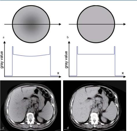
9.6 2D Artifacts

Fig. . . a, b Cupping artifact due to beam hardening and the result of water correction for a skull phantom and c, d for an axial abdominal tomogram (c, d: Courtesy of Siemens Medical Solutions)

More precisely, Fig. . a illustrates the consequences of an uncalibrated reconstruction. The cupping artifact is schematically reproduced for a simple head phantom, which consists of a high absorbing skull and a water-like X-ray absorbing soft tissue. The center gray-value proﬁle shows a sagged line, which may indicate an area being a ected by pathology. After water correction has been carried out, the center gray-value proﬁle should be a straight horizontal line as illustrated in Fig. . b. In Fig. . c and d the real reconstruction of an abdominal slice without and with water correction respectively can be seen.

However, this a priori correction cannot be performed for any potentially unknown object with arbitrary attenuation spectra, which di er considerably from those of water. Even if water correction has been carried out, beam-hardening artifacts might therefore occur in the area of thicker bony structures. This is illustrated

9 Image Quality and Artifacts

Fig. . . Streak artifacts in the base of the skull caused by beam hardening. The arrows mark the most peculiar image errors, which are due to the change in the X-ray spectrum while the beams pass through thicker bony structures. The shadow between the petrous bones is called the Hounsﬁeld bar. Since ﬁltered backprojection was used as a reconstruction algorithm, image errors spread from the structure, causing this error across the entire image

in Fig. . , which provides two CT reconstructions of the skull base, where socalled Hounsﬁeld bars, sometimes also referred to as interpetrous lucency artifacts, emerge between the petrous bones. These image errors are marked with arrows in Fig. . .

However, it would be possible to reconstruct images without beam-hardening artifacts with any wavelength or energy of radiation. Due to the speciﬁc attenuation property of the di erent tissues, a slightly di erent image would be produced for each individual energy. Due to this variety of information provided by images obtained with the above method, their combination might be useful in diagnostics. However, CT scanners do not produce monochromatic radiation. Nevertheless, the energy-dependent attenuation properties of the tissue are used in practice by scanning the patient with di erent accelerating voltages . With these images it is for instance possible to estimate the mineral content of bones and to compute images that look as acquired with monochromatic radiation. This allows an elegant beamhardening correction. In the dual-energy approach, the energy dependence of the attenuation coe cient must be modeled as

μ(ξ, η, E) = kabsorption(ξ, η) ċ αabsorption(E) + kscattering(ξ, η) ċ μscattering(E) .

( . )

Here, the spatial and energy dependence of the attenuation is factorized for the two main photon–matter interactions in the diagnostic energy window, i.e., photoelectric absorption and Compton scattering (cf. Sect. . . ). The energy dependence

In conventional ﬂuoroscopy, this method is also known as the dual-energy method.

9.6 2D Artifacts

of the photoelectric absorption is given by ( . )

αabsorption
αabsorption	(hν) .	( . )

The energy dependence of the Compton scattering is given by the Klein–Nishina equation ( . ), i.e.,

= ċ

+ E

( + E)

−

( + E)

−

+ E

πre

( .

μCompton n

( +

)

where E = hν (me c ) is the reduced energy of the incoming photon and n is the number of target atoms per unit volume. If ( . ) is substituted into ( . ), one obtains

pγ (ξ) =

= −

Emax

(

)

e−

(

)ċ

(

)ċ

(

∫ I

kabsorption

ξ,η

αabsorption

kscattering

ξ,η

μscattering

dη

dE!

∫

Emax

= −

(

)

e−

(

)

(

)

−

(

)

(

)

∫ I

αabsorption

kabsorption

ξ,η

dη

μscattering

kscattering

ξ,η

dη

dE!

∫

= −

Emax

(

)

∫ I

e−αabsorption

(E)Kabsorption(ξ)−μscattering (E)Kscattering (ξ)dE

( . )

where

Kabsorption(

ξ) =

∫ kabsorption(ξ, η)dη

( . )

and

Kscattering(ξ) =

∫ kscattering(ξ, η)dη .

( . )

The integrals Kabsorption(ξ) and Kscattering(ξ) can now be approximated by dualenergy measurements. That means, for instance, two di erent scans may be carried

9 Image Quality and Artifacts

out at two di erent X-ray tube voltages . T his leads to

	(		) = −			Emax		(		)	"
	(		) = −					(		)	"
p ,γ		ξ		ln		∫	I		E		e−αabsorption(E)Kabsorption(ξ)−μscattering (E)Kscattering(ξ) dE!
p ,γ		ξ		ln	I	∫	I		E
											#
											( . )

and

	(		) = −			Emax		(		)

p ,γ		ξ		ln		∫	I		E		e−αabsorption(E)Kabsorption(ξ)−μscattering (E)Kscattering
					I

where

I =	Emax	I (E)dE	and I =	Emax	I (E)dE .
	∫			∫

(ξ) dE" ,

( . )

Obviously, two projection integrals, p ,γ (ξ) and p ,γ (ξ), are measured for two un-

known variables Kabsorption (ξ) and Kscattering(ξ). In this way, the integrals Kabsorption and Kscattering can be estimated and, further, the distributions kabsorption(ξ, η) and kscattering(ξ, η) can be obtained by inverting the integrals ( . ) and ( . ) using the reconstruction methods from Chap. . Knowing the distributions kabsorption(ξ, η) and kscattering(ξ, η) in ( . ), artifact-free images can be reconstructed in an energy range that is correctly modeled with ( . ) and ( . ).

9.6.3

Motion Artifacts

So far it has been assumed that the morphology in the slice to be reconstructed is not changed during data acquisition. But if one also has to take into account the temporal variation of the attenuation coe cient, μ = μ(ξ, η, E, t), one faces the problem of image reconstruction with a changing data basis. That is, the data measured during the rotation are inconsistent.

One example of the occurrence of system-inherent or deliberately accepted inconsistencies is the spiral CT method, which has already been described in Sect.. . Due to the continuous table feed, none of the measured projection proﬁles consistently matches the other ones. However, as one knows the speed of the change, one is able to complete the spiral CT data by interpolation – within certain limits. These limits refer to the pitch factor. How image reconstruction is impaired if the selected pitch factor is too high will be described later in this chapter.

Split detector and sandwich principles or alternating X-ray tube voltages during rotation of the sampling unit have been proposed as well (Kak and Slaney ).

9.6 2D Artifacts

Another example of deliberately induced changes is the administration of contrast medium. If the absorption of contrast medium is to be observed dynamically, then the spatial distribution of the attenuation coe cient with respect to time also changes – however, this is exactly the physiological information one is interested in. But with regard to the imaging quality, there are also unwanted motions such as colon peristalsis, respiration, and the beating heart, which result in inconsistent projection data.

Figure . shows the simulation of the administration of contrast medium. A Perspex bar is introduced during a rotation into the central hole of a Perspex cylindrical phantom with ﬁve holes. In order to ensure that this change occurs in the projection angle interval ranging from to , a robot is used to introduce the Perspex bar into the plane that is to be reconstructed. The slice thickness is restricted to mm by means of collimators. Figure . b shows the sinogram with the detector data given as a function of the projection angle. The di erent holes of the phantom can be readily distinguished by the corresponding sine curves in the diagram – they are numbered accordingly. The correspondence is illustrated in Fig. . c, which provides the reconstructed image free from any motion artifacts. In order to be able to compare the di erent reconstructions, Fig. . e shows the image with the completely inserted central bar. This image does not show any motion artifacts either. The reconstruction corresponding to the sinogram of Fig. . b is shown in Fig. . d. The artifacts, spread over large image areas in a way that is characteristic of the backprojection method, are readily visible.

Recently, a data-driven method has been proposed that learns the motion parameters from the raw data (Schumacher and Fischer ). It combines the reconstruction and the motion correction in a single step. Such an augmented reconstruction can be formulated as a regularized optimization problem

(

)

f, ω

min

Ai T

(

ωi

)

−

αR

(

( . )

f Ω

The number K denotes the number of projection sets where the object is at rest. The system matrix Ai , which models the projection geometry and the projection pi , is partitioned into K sets. Compared with the equations in Sect. . , the novel step within ( . ) is the introduction of the motion parameter ω describing the transformation T. Since ( . ) represents an over-determined system of equations, the image f and the motion parameters ω can be estimated by means of a leastsquares minimization.

However, one fundamental goal for engineers developing new CT scanner generations is the acceleration of the data acquisition process, particularly with respect to the time constants related to anatomical and physiological motions. The presently used scanners are multi-slice sub-second CTs, which, however, are not able to display perfect radiographs of beating hearts without ECG triggering.

The acquisition speed cannot be arbitrarily increased at present due to technical restrictions. On the one hand, the mechanical equipment reaches the load limit to

9 Image Quality and Artifacts

Fig. . . Simulation of the administration of contrast medium. During a rotation of the sampling unit, a matching Perspex bar is introduced into the central hole of a cylindrical Perspex phantom with ﬁve holes. a The bar is introduced by means of a robot pushing the bar into the hole while the sampling unit rotates by , starting with a projection angle θ = . b The sinogram shows the raw data of this measurement for a rotation about . On the ﬁrst half of the sinogram the ﬁve holes can be readily distinguished and are numbered accordingly. Beyond an angle of θ = the central hole fades more and more over an angular interval of (this corresponds to the partial volume e ect over a slice thickness ofmm) and then disappears. The tomogram corresponding to this sinogram is shown in d. Due to the inconsistencies related to the backprojection, this artifact is not limited to hole “ ” into which the bar has been introduced, but extends over wide image areas. To be able to compare the di erent models, the tomograms without artifact – c without bar and e with completely introduced bar – are also shown. c also shows the correspondence between the ﬁve holes to the sine curves in the sinogram given in b

be taken into account with the high angular velocities and the corresponding angular moments of a , -kg gantry. On the other hand, data transmission from the rotating sampling unit to the ﬁxed gantry is a bottle neck due to which the data rate cannot arbitrarily be increased as well. Electron beam computed tomography (EBCT) described in Sect. . is therefore still the technology providing the shortest acquisition times. However, recently, it has been claimed that a dual-source CT system, which will brieﬂy be discussed in Sect. . , actually achieves comparable acquisition times.

9.6 2D Artifacts

9.6.4

Sampling Artifacts

In Sect. . it has already been pointed out that, as in general in any signal processing task, Shannon’s sampling theorem must not be violated in CT. This applies to both the reconstruction of an axial slice and the subsequent reconstruction of D data presentations by slice stacking. Sub-sampling of a signal also results in the typical aliasing artifacts. The inherent sampling problem discussed in Sect. . arises particularly for the detector array with a rectangular sensitivity proﬁle of the single detector elements. That is, the individual elements would have to be arranged at half the distance of their own width. As this requirement cannot be met due to obvious technical reasons (cf. Sect. . ) one makes use of an elegant mechanical trick. The corrective action, which is nowadays used to prevent aliasing, is either the quarter detector shift or the so-called ﬂying focus of the X-ray tube.

9.6.5

Electronic Artifacts

There are several electronic defects deteriorating the image and in most cases destroying it. The most famous, or better, most notorious, electronic defect is the failure of a detector channel. In third-generation CT scanners such a detector defect will result in prominent so-called ring artifacts.

Figure . outlines the occurrence of the ring artifacts. As the X-ray source and the detector array are tightly joined at the sampling unit, the failure of an individual detector element or the corresponding processing channel respectively be-

Fig. . . In third-generation CT scanners, each detector element is responsible for the data collection on a circle in the object space. If one element fails, the data may only be acceptably reconstructed within the corresponding circle

9 Image Quality and Artifacts

Fig. . . Example of a detector channel failure. a The planning overview of an anthropomorphic torso phantom shows a defective detector as a straight vertical line resulting from the ﬁxed position of the X-ray tube while the table moves forward along the feed direction. The dashed horizontal line marks the location of the axial tomogram to be measured. b The sinogram also contains a straight line since the corresponding detector position ξn is shown as a function of the projection angle. The horizontal detector position indicates the defective channel. This position is not changed while the sampling unit rotates. The ﬁgures on the right side exemplarily show the image reconstructions with c a normal detector array and d a defective detector array. It is readily visible that only the image data located inside the corresponding circle, which is called the ring artifact and results from the tangents of the backprojected erroneous signals, are reconstructed without major errors

comes speciﬁcally visible. During the ﬁltered backprojection the virtual lines connecting the corresponding detector element and the X-ray source, which sometimes are called defective beams, form the tangents of a circle. This means that all values outside the circle are seriously concerned by this artifact. Inconsistencies with the measured values of the corresponding other projection directions in fact arise for each point of each line. Due to the backprojection, all image areas are again a ected by the artifact. However, the area inside the circle encounters

9.6 2D Artifacts

this problem less frequently (cf. Fig. . ). It is in fact possible to reconstruct the image almost without artifacts inside the circle formed by the defective beam tangents.

Figure . provides an example of the failure of a detector channel while an anthropomorphic torso phantom is scanned. In Fig. . a the planning overview of the phantom can be seen. T he axial slice is to be reconstructed along the gray dashed line through the heart. In the planning overview, it can be already seen that one of the measuring channels is defective. Due to the ﬁxed anterior-posterior orientation of the X-ray tube/detector array unit, the defective channel results in a straight line along the table feed direction.

Figure . b shows the Radon space as a sinogram. Although the sampling unit rotates over with approximately Np = , angular steps, the defective channel still stands out as a straight line. This can also be easily understood as the horizontal lines ξn = const. always correspond to a ﬁxed line connecting the radiation source and the detector array elements. Figure . c ﬁrst shows the artifact-free axial tomogram of the axial slice indicated with a dashed line in Fig. . a. Figure . d illustrates the consequences of the detector failure on the reconstruction process. The circle or ring is formed by accumulation of the circle tangents, which are backprojected over the entire image over . The generation principle of this ring artifact had already been illustrated schematically in Fig. . . Outside the circle the image is defective. Di erent Moiré patterns, which arise during reconstruction according to the number of the measured projection angles, Np, can be observed.

As already mentioned above, the result of the reconstruction process inside the ring is almost artifact-free. However, smaller waves are visible in the vicinity of the ring artifact inside the circle, which are also reconstruction artifacts. These waves are due to the convolution of the projection signal before it is backprojected. As a result of the convolution, the error in the ﬁltered projection is ﬁnally broader (cf. Fig. . ) than in the raw projection. However, the data error quickly decays with increasing distance from the circle toward the circle center.

9.6.6

Detector Afterglow

Images can also deteriorate due to too long a glow time of the X-ray detectors. The ﬂuorescence time of the detector material after conversion of an X-ray quantum into a visible photon should be as short as possible. Otherwise, afterglow artifacts appear in the reconstruction, which manifest as smeared object boundaries in the image. Although afterglow is a short-term e ect, it becomes signiﬁcant at the high rotation speed of the sampling unit. Afterglow is usually modeled as a linear e ect on the intensities, independent on the detector element position. It decays exponentially and, if the temporal signature is known, the artifact can be suppressed by means of deconvolution.

9 Image Quality and Artifacts

9.6.7

Metal Artifacts

One known problem in CT is the appearance of metal artifacts in reconstructed CT

images. Low-energy X-rays are attenuated more strongly than high-energy X-rays
(cf. Sect. . . ). Recall that the absorption is given by
α Z λ .	( . )

Due to the Z dependence, this beam-hardening e ect is prominent for metals that are introduced into the human body, such as dental ﬁllings or hip prostheses, and leads to inconsistencies in the Radon or projection space. These inconsistencies observed in the integral attenuation values are due to the polychromatic X-ray spectrum produced by the X-ray tube. Additionally, without applying the dual-energy principle, the total attenuation of the X-ray intensity is an a priori unknown combination of the photoelectric e ect and the Compton e ect. This often leads in the reconstructed images to artifacts in the form of dark stripes between metal objects with light, pin-striped lines covering the surrounding tissue. Besides beam hardening, another origin of the metal artifacts is a higher ratio of scattered radiation to primary radiation, causing a low SNR in the metal shadow. This e ect will be discussed in the subsection below. Additionally, the partial volume e ect ( Sect. . . ) is a source of metal artifacts in transmission CT images. Especially in those cases in which the radiation is completely absorbed due to the thickness of the materials, very bright strips are found radially around the object; thus, the complete image loses its diagnostic value.

If there are materials with high attenuation coe cients in the object to be examined, then strong streak artifacts arise, which are spread across the whole image. In practice, the system detects an inﬁnitely high attenuation coe cient of the object. In the reconstructed image, one obtains on the backprojection lines through the object extremely high numerical values, which are spread across the entire image, as already stated above, and more importantly may not be compensated for by any other projection direction. But, as mentioned above, even if the radiation is not completely absorbed, the arising beam-hardening artifacts and – due to the usually extended sharp-edged metal implant objects – partial volume artifacts are so strong that the diagnostic value is considerably reduced.

Figure . shows the occurrence of metal artifacts in the tomographic reconstructions of the dental area. Figure . a again shows the planning overview scan on which the position of the slices to be measured is selected. Figure . b–d shows three axial reconstructions. Major artifacts are not visible in Fig. . b; however, on Fig. . c and d, it can be seen that bright strike artifacts arise with an increasing quantity of highly absorbing substance (in the tooth area this is frequently amalgam) through which the radiation must obviously penetrate inside the slice to be

From a physical point of view, due to ( . ) the radiation is of course never completely absorbed. But in practice the intensity may drop below the sensitivity of the detector or the noise level may be higher than the signal level.

9.6 2D Artifacts

Fig. . . Metal artifacts in CT images of a jaw. a presents the overview scan used to plan the axial slices. b–d then show the axial reconstructions at di erent slice positions throughout the tooth area. It is readily visible that the metal strike artifacts are considerably increased with the solid amalgam tooth ﬁllings

reconstructed. Along the lines connecting di erent ﬁllings, the artifacts are particularly striking, because the radiation must then pass through two metal volumes. The fact that the artifacts occur star-like around the metal object is a result of the principle of the ﬁltered backprojection. Since the physical origin of the artifact is always located in the respective X-ray path of the backprojection under the diverse angles, the streaks appear radially distributed around the origin.

Although the mechanism is clear, standard ﬁltered backprojection does not cope with these inconsistencies in the integral attenuation values. Thus, artifacts emerge within ﬁltered backprojection, because the Radon space values are inherently considered as a complete set of consistent absorption integrals of a monochromatic process.

9 Image Quality and Artifacts

On the other hand, statistical reconstruction techniques (cf. Chap. ) are especially capable of dealing with the metal artifact reduction problem. The core of these methods consists of an a priori knowledge of the statistical distribution of photon counts and a system matrix that models the physical X-ray absorption process. Each row of the system matrix represents a single X-ray beam running through the measurement volume. Contrary to ﬁltered backprojection, the inﬂuence of each single beam on the image reconstruction can be weighted separately. In this way, beams through the metal objects can be treated appropriately.

Within the maximum likelihood (MLEM) algorithm discussed in Chap. , the image f is estimated that best ﬁts the measured projections p under consideration of the statistical photon-count variations. It is based on the realistic assumption that the photon counts follow a Poisson process. The parameters of the joint Poisson distribution, which resemble the expectations of the linear attenuation coe cients of the CT image f, have to be estimated from the measured projection data. T hanks to the exponential Lambert–Beer attenuation law, the photon count is coupled to the attenuation values that form the image f. Therefore, the MLEM algorithm is generally superior to the ﬁltered backprojection with respect to streaking artifacts in the reconstructed image. This is due to the fact that, generally, MLEM for transmission CT

							N
						M	− ai j f j (n)
fr (	n	+	) = fr (	n	)	7	air e j =	( . )
fr (		+	) = fr (		)	7	iM air e−pi	( . )
						i =
							7
							=

has an inherent weighting. Any X-ray that intersects a metal object will naturally have a low intensity value. So, such rays will automatically get less weight, because the projection integral

	N
pi	=	ai j f j	( . )
	j =

of the estimated forward projection and the actual measured projection value pi weight the inﬂuence of the corresponding terms in the sums of the nominator and denominator respectively in ( . ). This is due to comparably high values of pi and pi .

However, inconsistent projection data can also be repaired with surrogate data created by interpolation or the inconsistent data can be treated as missing data in order to ignore the inconsistent data in the statistical approach . T he problem with the interpolated surrogate data is that these always include residual inconsistencies due to missing information during interpolation. On the other hand, within the missing data approach, a brute force method is applied to eliminate inconsistencies. However, the problem with this strategy is that the reconstruction actually su ers

This is not possible for a ﬁltered backprojection based reconstruction.

9.6 2D Artifacts

from voids in the projection data. Recently, it has been shown (Oehler and Buzug) that both strategies may be combined. A weighted MLEM approach can be used to reduce the inﬂuence of the residual inconsistencies from interpolation in such a way that optimal imaging quality is obtained by optimizing the compromise between residual inconsistencies and void data.

Fig. . . a Philips CT scanner with CIRS torso phantom marked with steel markers. b Sinogram of the torso phantom marked with two steel markers. c Region of interest from the sinogram (b). Di erent interpolation methods displayed in the region of interest. d Interpolation inside one projection under one angle; e directional interpolation. f,g Reconstruction of torso phantom data. f λ-MLEM reconstruction with linear interpolation and g λ-MLEM reconstruction with directional interpolation (Oehler and Buzug )

9 Image Quality and Artifacts

Raw data of an anthropomorphic torso phantom marked with two metal markers in a certain slice were acquired (cf. Fig. . a). Flat metal cylinders with a diameter of mm and a height of mm – similar to those used as ﬁducial markers in image-guided surgery – are used as markers in the experiments. The markers are made of steel of high atomic number. This leads to an ampliﬁcation of the beamhardening artifact, introducing inconsistent raw data. The markers are placed outside the phantom, because this conﬁguration ensures that the sinusoidal metal trace inside the Radon space has a maximum amplitude crossing all other sinogram structures of the phantom. This is the most complicated case for evaluating the interpolation. In Fig. . b the sinogram data of the torso phantom equipped with the steel markers are shown.

In a ﬁrst step, inconsistent projection data are bridged by interpolation. For this, the metal object is labeled in a preliminary ﬁltered backprojection reconstruction using a simple threshold. Subsequently, a forward projection of the metal-marker image is calculated, resulting in metal-trace projection data. This is used to label the projections running through a metal object, i.e., the metal traces shown in Fig. . b.

To demonstrate that di erent interpolation methods lead to di erent results in terms of metal artifact reduction in the reconstructed images, the inconsistent data are bridged by two di erent interpolation methods. The ﬁrst is the standard method (Glover and Pelc ): A linear interpolation inside one projection under one ﬁxed view is used (Fig. . c,d: Interpolation at an angle of between q and ). The second method, which considers the arrangement of the underling raw data, is a directional interpolation ﬁlling the gaps of inconsistent data following the ﬂow of the sinogram data outside the metal traces. The principle of directional interpolation is shown in Fig. . c, e (interpolation between r and s). This method leads to superior results compared with the ﬁrst interpolation schemes. Due to interpolation, the projection values of the soft tissue lying behind the metal markers are estimated.

Unfortunately, any interpolation-based repair scheme of the Radon space is based on a weak underlying physical model and hence it cannot be expected that the estimated projection data will perfectly ﬁt the projection data measured without metal markers. Therefore, projections pi running through a metal object, as well as the corresponding rows of the system matrix A = ai j , have to be weighted by an appropriate conﬁdence parameter λ . Recall that j ; , . . . , N corresponds to the number of image pixels and i ; , . . . , M to the number of projections. A careful choice of the conﬁdence parameter λ optimizes the compromise between residual inconsistencies and void data. The corresponding ﬁxed point iteration is given by

							N
						M	− λi ai j f j (n)
fr (	n	+	) = fr (	n	)	7	λi air e j =	.	( . )
fr (		+	) = fr (		)	7	iM λi air e−λi pi	.	( . )
						i =
							7
							=

9.6 2D Artifacts

T his modiﬁed MLEM algorithm is calledλ-MLEM (Oehler and Buzug ). Figure . f and g display the results of the di erent interpolation methods – linear interpolation (Fig. . f) inside one projection under one single view and directional interpolation (Fig. . g) – as a pre-processing step with consecutive λ-MLEM reconstruction. An appropriate weighting λ depends on the interpolation scheme and the size of the metal object. Linear interpolation is a frequently used approach to bridge metal data. It can be seen that this strategy works for the main artifact between the two markers.

However, strong new artifacts are introduced that stem from a sharp nondi erentiable connection between the measured and interpolated Radon space data. A directional interpolation follows the ﬂow of the Radon space (cf. Fig. . c). Contrary to the vertical interpolation schemes, the ﬂow consists of sinusoidal traces that connect projection values of actual objects inside the image. Consequently, better results are achieved with the λ-MLEM algorithm in combination with directional interpolation of the inconsistent data. As a practical rule of thumb, it has been recommended to set the parameter of the approach to λ = . . This always improves image quality compared with pure interpolation or missing data concept.

9.6.8

Scattered Radiation Artifacts

In Sect. . . the photon–matter interaction mechanisms of X-rays have already been discussed in detail. Whereas for the detector element located in the unscattered, direct beam path it does in principle not make a di erence which physical mechanism of the interaction actually reduces the intensity, as long as

( ) = −			(	s	) =
		I		s
p s	ln	I	( )

s
∫ μ(η)dη	( . )

holds (cf. ( . )). Other detector elements located outside the direct line of sight may in fact be impaired by certain interactions. Particularly in the area of strong attenuating anatomical objects such as the shoulder, abdomen, and pelvis (Morneburg ), the measured values may be distorted due to scattered radiation. These scattered X-rays may become a considerable part of the overall signal.

Whereas the scattered radiation is almost the same for all projection angles, it is very di erent for the wanted signal. In projection directions in which highly absorbing objects are located one after another, the wanted signal may become extremely weak so that the scattered radiation dominates the signal (cf. Fig. . a). Within the ﬁltered backprojection, inconsistencies then arise from this projection direction, which result in streak artifacts.

With regard to the interfering radiation caused by scattering reaching the detector, the third-generation CT scanners are superior to the fourth-generation CT scanners. Figure . b and c outlines the scanners of both generations. Figure . b shows the third-generation scanner. The detector array of this scanner is designed

9 Image Quality and Artifacts

Fig. . . a The background scatter signal may cover the wanted signal. Comparison of b the third and c the fourth generation of CT scanners with regard to their radial geometry. As the detector array of the third generation represents a circle segment, the center of which is located in the X-ray tube, it is possible to design an anti-scatter grid with septa pointing toward the X-ray focus

such that the row of detector elements is arranged on a circular segment whereby the X-ray source is located in the circle center. It is therefore possible to collimate the radiation by septa so that scattered radiation – with an incident angle into a “false” detector element, which is larger than a threshold angle – is e ectively shielded. The critical angle is determined by the length and the spacing of the detector segments.

9.7 3D Artifacts

Fig. . . The anti-scatter grid at the detector array; here the mobile Philips Tomoscan M – a third-generation scanner – is shown. The septa of the grid are readily visible in the close-up

In the fourth-generation scanners (c.f. Fig. . c) the detectors are located on a circle, the center of which is the iso-center of the measurement ﬁeld. An X-ray source, to which a detector collimation might be focused on successfully, obviously cannot be located there. Figure . shows the segmented scattered radiation grid at the detector array of the mobile CT scanner Philips Tomoscan M – a thirdgeneration scanner.

9.7

3D Artifacts

In connection with the so-called secondary reconstruction of three-dimensional images based on CT image stacks , but also with the implementation of D acquisition techniques such as spiral CT, cone-beam reconstruction, and their combinations – the spiral or helical cone-beam reconstruction – a variety of new artifacts may arise, which will only brieﬂy be discussed in this section.

In the form of multiplanar reformatting (MPR) or surface rendering.

9 Image Quality and Artifacts

9.7.1

Partial Volume Artifacts

Partial volume artifacts due to the ﬁnite detector width arise inside an axial slice. These artifacts, which have been discussed in Sect. . . , are called transversal partial volume artifacts. In addition, artifacts must also be expected in the axial or z direction, i.e., the table feed direction, due to the ﬁnitely collimated slices. These artifacts are called longitudinal or axial partial volume artifacts (Morneburg ). Figure . shows that averaging plays an important part, not only within one slice, but also in the axial direction due to the restricted slice thickness z.

In regions with a multitude of details rich in contrast, the partial volume artifacts may considerably disturb the reconstruction process. The slices in these anatomic regions should therefore be as thin as possible. Figure . demonstrates this e ect.

Even if the slice thickness is usually given by a single scalar value, one must bear in mind that X-rays are leaving the focal spot of the X-ray tube in all directions (cf.Chap. ). In this way, a source-sided collimation does not actually deﬁne a “slice thickness,” but rather the aperture angle of the fan beam in the longitudinal or axial direction. Figure . a shows the beam geometry for a thick slice and Fig. . b

Fig. . . Object boundaries passing through an axial slice with a high slope are blurred (schematically on top of the ﬁgure). a This e ect is readily visible in the area of the jaw. The arrows in the slices b and c indicate the blurred image areas

9.7 3D Artifacts

Fig. . . Longitudinal or axial partial volume artifact. a If the axial aperture of the X-ray fan beam is comparably large, di erent information (indicated by an arrow) is measured from the anterior–posterior (a.p.) and the posterior–anterior (p.a.) direction. b This leads to inconsistency artifacts in the reconstruction. c The amount of inconsistency can be reduced by a ﬁnely collimated X-ray beam. d In this way, the artifacts in the reconstruction are reduced

that for a ﬁnely collimated slice. Due to this reason, the projection measurements always carry inconsistencies to some extent.

However, these inconsistencies are particularly disturbing if the axial aperture angle is large and the object information is of high contrast. Bony structures, for instance, indicated with an arrow in Fig. . a, show highly contrasted structures

9 Image Quality and Artifacts

that are included in the measurement only in the anterior–posterior (a.p.) direction. As a consequence, the typical streak artifacts are visible in the reconstruction displayed in Fig. . c. As a counter-measure, the beam may be collimated ﬁnely (cf. Fig. . b) and the corresponding artifacts will be reduced (cf. Fig. . d).

9.7.2

Staircasing in Slice Stacks

If fast changes in object boundaries rich in contrast along the table feed direction arise in the object to be imaged, then steps can be encountered side by side in the three-dimensional reconstruction, leading to a stair-like appearance in the object visualization. These steps are artifacts produced by averaging the object boundary within the sensitivity proﬁle of the axial slice. Figure . shows this e ect schematically. At the skull surface visualization (cf. Fig. . d; the slice stack is also shown

Fig. . . If the object in the CT scanner is deﬁned by boundaries that steeply pass through the individual slices (a), then averaging within one slice (b) results in staircasing of the threedimensional reconstruction of the slice stack (c and d). Upper rows: Slice stack of the skull. The last four slices are assigned to the three-dimensional reconstruction with numbers

9.7 3D Artifacts

in the two top rows of this ﬁgure), it can be seen that the steps in the area in which the surface is subjected to considerably fast changes with respect to the axial (in this ﬁgure vertical) z direction are particularly pronounced.

This image error may be reduced by arranging very small collimated slices that potentially overlap. However, the more elegant method is the spiral CT approach, by means of which this artifact type may be e ectively reduced. In principle, arbitrarily dense slice stacks may be computed retrospectively with the method described inSect. . . In the case of fast changes in structures that are rich in contrast along the axial direction, a pitch factor p (cf. Eq. . ) smaller than is recommended (Blanck

Figure . shows the staircasing artifact on the images of a spine phantom. The individual slices scanned with conventional CT acquisition technology are mm thick here. This ﬁgure should also be compared with Figs. . and . in the previous chapter. The staircasing e ect, which expresses the anisotropy of the underlying data set, is particularly problematic if very small details must be analyzed.

Fig. . . Three-dimensional reconstruction of a vertebral phantom. Typical orthogonal reformatting and volume rendering can be seen. The slice thickness selected for the measurement is mm. The staircase pattern of the three-dimensional rendering and of the coronal and sagittal slices can be clearly seen

9 Image Quality and Artifacts

Fig. . . Comparison of the reconstruction quality of a spherical tumor phantom with a radius of mm. a shows the typical result of a conventional clinical CT system. The length extension of the sphere in the z direction is due to averaging within the slice. b shows the reconstruction result of a prototypical volume CT equipped with a ﬂat-panel X-ray detector with . mm isotropic spatial resolution (courtesy of General Electric Medical Systems: Pfoh [ ])

Figure . shows the image of a spherical tumor phantom with a radius ofmm. Figure . a demonstrates the typical length extension of the object due to averaging within the slice measuring . mm thick. Inside the slice the resolution is of course better and amounts to approximately . mm in this example. In the isotropic presentation acquired with a volume or cone-beam CT with a spatial resolution of μm, in Fig. . b the spherical shape of the phantom is revealed. Therefore, errors with regard to the volume estimation in tumor studies can be reduced. The considerably higher spatial resolution with the cone-beam system does in consequence not only enable a more precise quantitative volume measurement, but also the potential early detection of small tumors in oncology (Pfoh ).

9.7.3

Motion Artifacts

Motion artifacts in a two-dimensional image, i.e., in the reconstruction of a single axial slice, have already been described in Sect. . . . In the two-dimensional case, image errors such as streaks, blurring, and ghost images found in the backprojection were particularly due to inconsistencies in the raw data, i.e., the data of the Radon space.

Another problem now arises with the three-dimensional, secondary reconstruction, in which the size and position of objects to be imaged by several axial slices in a stack no longer match with regard to the original object in consecutive slices. Figure . shows one example in which the data set is blurred by respiration. On the upper left of the ﬁgure, in the three-dimensional visualization of the

9.7 3D Artifacts

Fig. . . Motion artifacts in the three-dimensional reconstruction. After approximately three-quarters of all planned axial slices from the shoulder to the abdomen had been measured, the patient could no longer hold his breath. In the last quarter of the data set this resulted in o sets and blurring marked by arrows in the corresponding images (courtesy of Ruhlmann, Medical Center Bonn)

skin surface, it can be seen that the patient data in the lower quarter of the slice stack (see arrow) have body contours that do not match each other.

In this example, the patient was not able to hold his breath during the acquisition time. If one selects an axial view of such a slice blurred by respiration, this blurring e ect and the resulting ghost structures (marked by arrows) can readily be seen. The disturbances of course continue in the corresponding reformatting, i.e., in the calculated sagittal and coronal slices. The correspondence among the axial, sagittal, and coronal slice is indicated by vertical and horizontal lines in the images.

9.7.4

Shearing in Slice Stacks Due to Gantry Tilt

The spatial normal vectors of the individual slices need not necessarily match with the z-axis, i.e., the table feed axis of the CT system. Under certain anatomic conditions, the gantry, i.e., the frame of the rotating sampling unit with the X-ray tube and the detector array, must be inclined so that the relevant structures are located within one slice and need not be assembled from a slice stack. Figure . a and b shows the planning overview for a skull tomogram with two possible slice sequences. In Fig. . a, the normal slice stack is planned. This corresponds to the

9 Image Quality and Artifacts

Fig. . . Planning overview of a cranial tomogram. a, c Normal slice sequence; b, d angulated slice sequence. Due to the anatomical orientation of the brain inside the skull, the angulated slice sequences are more appropriate. The eyes are, for example, not exposed to direct radiation. The measured slice stack is shown in Fig. .

upright position of the gantry (cf. Fig. . c). In Fig. . b, an angulated slice sequence is planned. This corresponds to the tilted gantry shown in Fig. . d. Due to the anatomical orientation of the cortex inside the skull, an angulated sequence of images is frequently used to prevent unnecessarily high doses of direct radiation on the sensitive eyes.

Fig. . . Schematic sketch of the slice sequence of conventional data acquisition, not taking into account the sampling theorem. Left: Slice acquisition vertical to the z-axis. Right: Tilted slice acquisition

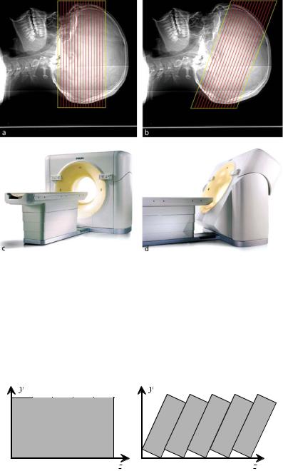
9.7 3D Artifacts

Figure . once again shows schematically the orientation of the individual slices with the normal and angulated form. If one wants to compose a slice stack measured in the angulated orientation of the gantry to provide a three-dimensional presentation, then the orientation of the data set must be corrected slice by slice. Figure . illustrates the correction process schematically and Fig. . shows the result on the skull tomograms presented in Fig. . as a slice sequence. Shearing does not only occur with an inclined gantry. When the table moves into the meas-

Fig. . . a If one assembles the data measured from an angulated slice sequence without any correction into a slice stack, b the individual slices will be sheared with respect to one other. c If one reverses this shearing process the data are available as they were in the original measurement (a). However, the image will not have a rectangular format. d If one corrects this deﬁciency by increasing the cyclic movement of the slices, e the object seems to be cyclically shifted. f This deﬁciency can be corrected in a last step – by synchronous cyclic shifting of all slices

Fig. . . If the skull measured with an angulated slice sequence is assembled by stacking one slice on top of another without any further corrective action, the single slices seem to be sheared with respect to one other. This is readily visible on the left-hand picture (cf. b in Fig. . ). Staircasing indicates the thickness of the slices. Shearing has been corrected on the picture in the center, but the object seems to be cyclically shifted (cf. e in Fig. . ). On the right-hand picture, the cyclic shifting has also been corrected (cf. f in Fig. . )

9 Image Quality and Artifacts

uring ﬁeld, the gravity moment acting on the table increases more and more the longer the path of the table through the gantry. This table deformation, the amount of which depends on the feed length, also results in shearing of the individual slices. However, this deformation is rather small and does not play a role at all with respect to diagnosis. But if the CT data are used for image-guided surgery, then the table deformation must be corrected (Zylka and Wischmann ).

9.7.5

Sampling Artifacts in Secondary Reconstruction

In Sect. . it has already been pointed out that the requirement given in Shan-

non’s sampling theorem must be met within an axial slice and in an axial direction

as well. Due to ( . ) the axial sampling points must therefore have a distance	z
from each other. This means that the table must not be moved by more than	z

when a slice thickness of z has been chosen. Thus, at least two slices have to be measured per slice thickness. Otherwise, the secondary reconstruction might be subjected to aliasing artifacts. Figure . demonstrates this aliasing e ect in a secondary reconstruction of an aluminum hole phantom.

Fig. . . Tomographic survey of a hole phantom (A phantom on the left-hand side) with a slice thickness of mm each. If a slice is acquired every z = . mm (center) or every z =. mm (right side) respectively, and a secondary three-dimensional reconstruction is carried out, aliasing artifacts in the horizontal hole grid with d = . mm (diameter = distance) can be seen

9.7 3D Artifacts

9.7.6

Metal Artifacts in Slice Stacks

If considerably strong artifacts arise within a slice, then this slice destroys the secondary three-dimensional reconstruction of the volume in this slice. Figure . shows the e ects of metal artifacts in the three-dimensional image. Looking at the

Fig. . . Metal artifacts in the three-dimensional reconstruction. The ﬁgures a through d show axial slices with artifacts of di erent strengths, depending on the number of tooth ﬁllings in the slice. e and f show a coronal and sagittal slice reconstruction (or reformatting) from an axial stack of slices respectively. The spatial orientations of this reformatting are always shown on the upper right on e and f. g and h show surface renderings based on a simple gray-value threshold in which one can readily see the metal artifacts in the corresponding axial slices (courtesy of Ruhlmann, Medical Center Bonn)

	9 Image Quality and Artifacts
	jaw tomography that has already been presented in Sect. . . , once again some
	axial slice reconstructions can be seen in the sequence of Fig. . a–d (anatomically
	from bottom to top). In Fig. . a one initially does not see any signiﬁcant artifacts.
	In Fig. . b one can readily see that two metal objects located in the beam path
	produce strong artifacts in the area of their connecting lines. In Fig. . c a multi-
	tude of tooth ﬁllings are located in the area of the slice to be reconstructed so that
	the whole image is completely degraded by streaks due to the inconsistencies of the
	projections from di erent directions. Figure . d once again illustrates the radial
	propagation of the streaks in the area of a single tooth ﬁlling.
	If one stacks the individual slices one above another, the image of a coronal
	slice (Fig. . e) and of a sagittal slice (Fig. . f) in orthogonal reformatting can
	be computed. The location of the corresponding slices is inserted in an artifact-free
	axial slice on the upper right-hand side. One can clearly see that the complete slices
	are contaminated with artifacts in the area of the tooth ﬁllings.
	Figure . g and h shows three-dimensional visualizations of the jaw. These are
	surface renderings based on gray-value threshold bone segmentations. Both ﬁg-
	ures show the same object, each with a di erent viewing angle. Outside the slices
	impaired by the tooth ﬁllings, the image quality of the tomogram is very good.
	9.7.7
	Spiral CT Artifacts
	In principle, image errors also arise in spiral CT that are similar to those arising in
	the direct reconstruction of single axial slices. However, these artifacts are generally
	not as strong as they are in single-slice CT, since spiral CT reduces considerably, for
	example, motion artifacts or staircasing in the secondary reconstruction. However,
	new spiral-related reconstruction artifacts arise with this CT method, which are
	mainly due to interpolation inaccuracies in combination with the selection of the
	pitch factor. In principle, one ﬁnds here as many image error types as interpolation
	methods. In this section, the interpolation problem cannot be discussed in detail,
	but the so-called scalloping (Blanck ) artifact should be mentioned, which is due
	to the fact that the slice sensitivity proﬁle is increased in spiral CT so that partial
	volume artifacts also become stronger (Wilting ).
	Scalloping is a phenomenon arising, for example, in skull tomographies, particu-
	larly in slice positions in which the skull diameter quickly changes its axial direc-
	tion. Figure . shows an example of this speciﬁc spiral artifact. Two slices with
	di erent curvatures in axial directions have been selected in a skull phantom. For
	comparison, the slices with a thickness of mm were measured for both positions
	conventionally, i.e., without a continuous table feed.
	The result is shown in Fig. . a and b. The virtually di erent thicknesses of
	the skull in the two slice positions is due to the fact that the angle between the
	corresponding reconstruction layer and the local skull surface normal vector varies.
	One can also readily see the partial volume artifacts arising as a thin fringe around
	the skull structure.

9.7 3D Artifacts

Fig. . . Interpolation artifact in spiral CT. Top: The data structure looks like a cut radish. On the lower left one sees the planning overview of a skull phantom in which two slices have been selected. a and b show the corresponding, conventionally acquired reconstructed slices with the partial volume artifacts described in . . and . . . These existing artifacts are overlaid by an interpolation artifact if an excessively high pitch factor is chosen. The stronger the curvature of the object in the axial direction, the more this error becomes visible in the corresponding parts c and d

If the spiral acquisition method is used in this geometrical situation, errors may arise with an excessively high pitch factor. These are shown in Fig. . c and d. The fringe around the bone structure is considerably enlarged and it is shifted as a function of the angular position of the sampling system. This fringe is due to the fact that data are used for interpolation that are not really close to each other due to the quick axial change of the skull structure. This e ect is usually small. To make it nevertheless noticeable, an excessively high pitch factor of p = has been chosen.

	9 Image Quality and Artifacts
	If the pitch factors are carefully selected, this image error will not be relevant in
	radiological practice. However, it is revealed in the reconstruction of this example
	that the data structure of the spiral CT resembles a helically cut radish (cf. Fig. . ,
	top).
	9.7.8
	Cone-Beam Artifacts
	Similar to the spiral CT method, a multitude of artifacts also arise with the cone-
	beam reconstruction method that cannot be discussed in detail here. All artifacts
	mentioned above may of course also occur with cone-beam geometry, even though
	some image errors such as motion artifacts may be reduced due to the increased
	acquisition speed. But again, new image errors arise with this method, which are

Fig. . . Result of the cone-beam correction with larger aperture angles of the X-ray cone. a–c show an anthropomorphic thorax phantom. c is the reformatted plane selected by the vertical line in b. An important factor inﬂuencing the quality of the cone-beam reconstruction is the adaptation of the reconstruction plane to the spiral geometry. d shows the corresponding reconstruction planes. The di erent reconstruction results are shown in e–g. e shows the

standard reconstruction for a			-mm slice with a feed of mm/s, f the standard recon-
struction for a	-mm slice with a feed of mm/s, and g the reconstruction with the
plane correction for a		-mm slice with a feed of mm/s (courtesy of Siemens Medical
Solutions)

9.7 3D Artifacts

for example due to the shadow zone of the Radon space in cases of incomplete data sets (Wang et al. ; Lee et al. ).

In practice, the choice of the orientation of the reconstruction plane within the helical cone-beam geometry is particularly important. Figure . a–c shows a simulation of an anthropomorphic thorax phantom.

Figure . d illustrates the adaptation of the inclination of the reconstruction plane to the cone-beam geometry and the Fig. . e–g illustrates the corresponding reconstruction results (Stierstorfer et al. ). The result of the reconstruction using the data of a -line detector with a slice thickness of mm each and a feed of mm s is still acceptable for clinical applications with standard reconstruction, although the cone aperture angle has not been taken into account (cf. Fig. . e).

However, the mathematical approximations of the standard reconstruction with regard to the actual inclination of the reconstruction plane in the three-dimensional space are no longer valid with larger cone aperture angles. The standard reconstruction therefore produces considerable artifacts if, for instance, a -line detector is used with a slice thickness of mm each and a feed of mm s (cf. Fig. . f). Figure . g illustrates that the image quality is considerably improved by adapting the reconstruction plane.

9.7.9

Segmentation and Triangulation Inaccuracies

The viewing workstation frequently presents very smooth surfaces to the clinician, which, however, does not allow a conclusion to be drawn regarding the parameters of the scan protocol, such as the slice thickness or the spiral reconstruction index. Figure . shows the visualization results for the vertebral phantom presented in Fig. . in the previous chapter. On the left-hand side a volume rendering is shown, in which the slice thickness can be clearly concluded from the ﬁgure. On the righthand side a surface rendering is shown, which does not give any indication of the

Fig. . . Result of the volume and the surface representation of a vertebral phantom. In the volume representation (left) the slice thickness of mm is evident. The surface rendering (right) does not give an indication of the slice thickness

9 Image Quality and Artifacts

Fig. . . Left: An iso-line is selected in the measured slice by an individually chosen grayvalue threshold. Center: Orientation of the measured slice in the data volume. Right: A stack of iso-lines of nine measured slices is the basis for triangulation

slice thickness. However, both representations are based on the same data acquisition protocol.

To understand why the slice thickness is no longer discernible in the surface representation, the visualization process must be brieﬂy discussed. Within the visualization process, the user may decide to show special ranges of gray values and to mask out other ones selectively. If the user selects a constant gray value as a threshold, then all spatial points with this gray-value attribute are displayed as iso-surfaces in space. A single iso-line within the selected slice is shown on the left-hand side of Fig. . . This example illustrates that the type of segmentation may already lead to errors. T he spinous processes, for example, which are more faintly imaged due to the partial volume e ect, are not enclosed by the iso-line. In the middle of Fig. . the location of the slice in the three-dimensional data volume is shown to improve the orientation. The right-hand side of Fig. . illustrates the stack of the nine measured slices with the individual iso-lines.

The stack of the iso-lines is the basis for visualization since the gray-value threshold-based iso-surface is reproduced with triangles on the basis of these lines. Figure . illustrates the result of the triangulation. The iso-surface is shown as a virtual surface by assigning each of the triangles with a reﬂectance and then illuminating the mosaic consisting of the triangle tiles with a virtual light source (Fig. . , right).

The higher the number of mosaic elements used to reproduce the surface, the more realistic the result. Approximately , triangles have been computed in Fig. . (right). In Fig. . , on the left-hand side, this result is compared with a densely acquired spiral CT scan. Between the iso-lines of slices that have been retrospectively computed with a distance of . mm, , triangles form the surface (dark shaded surface). The accuracy di erence becomes visible when the surfaces of the conventional nine-slice measurement are visualized within the same volume (bright shaded surface).

Figure . , on the right-hand side, illustrates once again why the result of the coarse measurement must be less accurate. The actual data basis is superimposed onto a transparent surface representation with a sagittal slice. The location of the

9.7 3D Artifacts

Fig. . . Left: Grid model for the triangulation based on the iso-lines. Right: Each of the triangles is assigned a reﬂectance and illuminated with a virtual light source

Fig. . . Left: The surface representations of the ﬁnely acquired spiral CT scan with retrospectively computed slices with a reconstruction distance of . mm (dark shaded surface) and a conventional measurement of nine slices with a slice thickness of mm (bright shaded surface) are compared. Right: The sagittal slice in the visualization of the transparent surfaces reveals the di erence between the coarse data basis and the smoothening triangulation

surface in space is obviously the result of an interpolation. Furthermore, the selection of the gray value threshold for the iso-surface is obviously subject to a certain arbitrariness and, in addition, the location of the surface is inﬂuenced by the partial volume artifacts. This must always be taken into account when planning a surgical intervention, for example, when so-called pedicle screws are to be placed through the spinous processes, so that the screws are always placed exactly at the planned location.

9 Image Quality and Artifacts

9.8

Noise in Reconstructed Images

To evaluate and quantify noise in the reconstructed images, the data acquisition chain has to be studied once again. At the end of the chain the CT images are in fact a superposition of ﬁltered projection data. However, the physical source of the noise is the measurement process of X-ray quanta and this process indicates the beginning of the signal processing chain.

In principle, noise must be classiﬁed into the categories of quantum noise and detector noise. The quantum noise is produced by stochastic ﬂuctuations regarding scattering and absorption while the radiation passes through the object. In spite of identical radiographic situations the number of quanta reaching the detector always varies.

This stochastic process is modeled by additive noise. The quantum noise level is linearly increased with the intensity. The quantum noise reveals that the energy is transmitted to the detector in small portions, the X-ray quanta. In contrast, detector noise is a thermal noise produced by the electrons in the detector, does not depend on the X-ray exposure, and above all can also be measured without radiation.

9.8.1

Variance of the Radon Transform

The noise analysis is started with consideration of the number of quanta on a single detector element. As the intensity of the radiation is proportional to the number of quanta measured in the detector, one ﬁrst takes into account Beer’s attenuation law – cf. ( . ) – which reads

nγ (ξ) = nγ, (ξ)e− ∫ μ(η)dη , ( . )

where nγ (ξ) is the number of quanta measured under the projection angle γ at the detector element ξ, and nγ, (ξ) is the reference number of quanta without any absorbing objects in the measurement ﬁeld. Due to the linear relation between the radiation intensity and the number of quanta, the projection integral – cf. ( . ) – can be given by

pγ (ξ) = − ∫	μ(ξ, η)dη = ln nγ		(ξ ) = ln nγ, (ξ) − ln nγ (ξ) .		( . )
		nγ,	ξ
The values of the projection integral represent( )				the Radon space. As the number of

quanta measured during the counting process is subject to Poisson distribution, the
average value `nγ (ξ)a and the standard deviation σn,γ (ξ) obey the relation
`nγ (ξ)a = σn,γ (ξ)	( . )

Recall that the mean value is an estimate of the expectation value.

9.8 Noise in Reconstructed Images

(cf.	Sect. . ), so that the measurement of the number of quanta on the individual

detectors can be expressed as
	nγ (ξ) = `nγ (ξ)a $ σn,γ(ξ) = `nγ (ξ)a $ c`nγ (ξ)a .	( . )

As the next step in the signal processing chain consists of the logarithmation of the values measured with the detector, one is interested in the standard deviation of the

projection integral pγ

ξ .

) in ( . ), one ﬁnds

If one substitutes (( .)

pγ (ξ) = ln nγ, (ξ) − ln `nγ (ξ)a $ c`nγ (ξ)a

nγ

nγ,

(

) −

nγ

(

)ag

(

( ) −

( )a k#

` ( )ag

( . )

ln nγ, ξ

nγ ξ

nγ

(

= ln nγ, (ξ) − ln `nγ (ξ)a + ln $

nγ

(

! .

With the series expansion

(% i)

)a#

i =

for

( . )

( $

) = −

−

< +

it can be concluded for `nγ (ξ)a and the truncation of the expansion ( . ) after the linear term that

pγ (ξ) = ln nγ, (ξ) − ln `nγ (ξ)a $	G		.	( . )
		`nγ (ξ)a

According to ( . ), the ﬁrst two terms in ( . ) can be considered as the average value of the projection integral such that


pγ (ξ) = `pγ (ξ)a $ G nγ ξ					.	( . )

The standard deviation of the projection		integral therefore obeys
The standard deviation of the projection		` (		)a
	σp,γ(ξ) =	G				( . )
and the variance is given by	σp,γ(ξ) =	G	`nγ (ξ)a			( . )
	σp,γ(ξ)
	σp,γ(ξ)	= `nγ (ξ)a .				( . )

9 Image Quality and Artifacts

9.8.2

Variance of the Reconstruction

The next step in the reconstruction chain considered here is the ﬁltered backprojection, which can be formulated with its discrete form – cf. ( . ) – as

f (x, y) = π p hγn (x cos(γn ) + y sin(γn )) . ( . )

Np n =

If the convolution is carried out in the spatial domain of the detector array to ﬁlter the projection signal, one can write, in analogy to ( . ),

(

) =

Np D −

(

)

(

) +

(

) −

)

x, y

pγn

k ξ

gγn

x cos

γn

y sin

γn

k ξ

. ( . )

n = k=−D

Taking into account ( . ), it can be seen that

(

) =

D −

(

)a $ G

x, y

ξ n = k=−D

pγn

k ξ

nγn

. . .

y sin

(

γn

) −

k ξ

)

(

	)a#	(		(		) +
ξ	! gγn		x cos		γn		. . .

( . )

so that the individual pixel values may compactly read

where

f (x, y) = `f (x, y)a $ σf (x, y)

( . )

`f (x, y)a =

D −

`pγn

ξ)agγn (x cos(γn ) + y sin(γn ) − k

ξ)

ξ n = k =−D

( . )

and

(

) =

D −

(

) +

(

) −

)

σf

x, y

(

gγn

x cos

γn

y sin

γn

n = k

−D

γn

( . )

As the individual projections represent statistically independent ﬂuctuations, the variance can be expressed as

(

) =

D −

gγn

x cos

γn

y sin

γn

k ξ

σf

x, y

(

( )a

) , ( . )

n = k

−D

n)γn+ k ξ

( ) −

because the mixed terms add up to zero.

9.8 Noise in Reconstructed Images

The variance in the origin is thus

D −

gγn k ξ

σf

(

) =

nγn (k ξ)

( . )

n = k =−D

since a comparison with

Sect. . . shows that

`g is(an even)a

function so that

(−

) =

(

)

cylindrical, homogeneous object, the ﬂuctuation of the

g k

ξ . For a

center beam is always the same under any projection angle; thus,

D −

(

) =

(

)

( . )

σf

n =

nγn

(

! k =−D gγ

k ξ

)a#

! .

D −

(

)

k ξ

k =−D gγ

If the general relation for integral`

(discretization,)a

i.e.,

ξ gγ (k

ξ) ∫ gγ (ξ)dξ

( . )

and, furthermore, Rayleigh’s theorem (cf. Sect. . ), is used, then the real signal gγ (ξ) obeys

∫ gγ (ξ)dξ = ∫ SGγ (q)S dq	( . )
and, thus, the variance of the pixel in the origin obeys

σf	( , ) = Np			ξ
			π
	=		π	ξ
	=	Np`n( )a


	+
Np	+			ξ
Np					SGγ (q)S
`n( )a		−	∫			dq
	ξ		∫			dq
			ξ				( . )

+ξ

∫SGγ (q)S dq .

−ξ

Obviously, the pixel noise of the reconstructed image depends on the selected ﬁlter function of the ﬁltered backprojection. The variance σf ( , ) of the pixel f ( , ) is proportional to the area under the quadratic norm of the ﬁlter functional in the frequency space. Several ﬁlter functions have been presented in Sect. . . If the functionals ( . ) through ( . ) are combined with ( . ), one clearly sees that the image noise can be reduced by minimizing the area


	+
σf ( , )			ξ	SGγ (q)S dq .
	−	∫			( . )
		ξ

Without restriction of generality, the behavior of the center pixel only is discussed.

9 Image Quality and Artifacts

On the other hand, it must be taken into account that any deviation from ideal ﬁltering

G(q) = q for all q ,

( . )

results in a reduction of the spatial resolution because, as mentioned earlier in this chapter, the MTF of the reconstructed image depends on the type of band limitation and windowing of the ideal linear ﬁlter function. In Sect. . it was explained that the spatial resolution is determined by

(	) =	(	)
MTFfilter kernel		G q
MTFfilter kernel	q	q	.	( . )
		q

This means that the spatial resolution cannot be maximized without increasing the image noise, too. The selection of the ﬁlter functional is an optimization process in which one has to ﬁnd a trade-o between acceptable image noise and the required spatial resolution, depending upon the anatomical problem. If ( . ) is substituted into ( . ) one ﬁnds the expression


		+
				ξ
σf ( , ) =	π ξ	−	∫		qMTFfilter kernel	(q) dq .	( . )
	Np`n( )a
			ξ

Minimizing the area under the integral would thus unfortunately mean that the MTF would be minimized.

If a ﬁxed ﬁlter functional G(q) is assumed, the normalization term

σf ( , )	π ξ			( . )
	Np	n
of ( . ) can be analyzed. Obviously, noise is`		reduced with an increasing number
		(	)a

of projections, Np .

Furthermore, ( . ) supports the impression that the width of the detector elements ξ must be kept as small as possible to achieve a small variance in the reconstructed pixels. This is actually a false conclusion since, on the one hand, the average number of quanta `n( )a, measured in one single detector element, linearly depends on the detector width. On the other hand, the width of the detector elements appears within the limits of the integral term of ( . ). Therefore, one has to solve this integral to draw a ﬁnal conclusion on the dependence of variance and detector width. For this purpose, ideal (rectangular) ﬁltering – cf. ( . ) – is assumed; thus, band limitation results in

` (

(

σf ( , ) =

∫

(q)

dq =

Pq Q− ξ

−

( . )

`n( )a

( ξ)

Np`n( )a( ξ)

9.8 Noise in Reconstructed Images

Fig. . . Inﬂuence of the radiation intensity and the number of projections on the noise in the reconstructed image. The phantom was scanned with di erent numbers of projections, Np, and tube currents, I (a: Np = , and I = mA; b: Np = and I = mA; c: Np = and I = mA)

In fact, the variance increases inversely proportional to the square of the detector width.

In ( . ), `n( )a is the mean number of transmitted X-ray quanta of the center beam. For a circular disk of radius R and homogeneous attenuation μ, this number can be estimated by

`n( )a = `n ( )ae	R	μ dη	= `n ( )ae− R μ .	( . )

	− ∫

Under any angle, the mean value of the quanta number reaching the detector is equal to the number of quanta generated in the X-ray source, multiplied by a constant attenuation factor. As the mean number of quanta `n( )a is inversely proportional to the variance of the image noise, the noise may obviously be reduced by increasing `n ( )a. The number of quanta `n ( )a depends on the current I of the X-ray tube (cf. . and . ). The higher the tube current, the higher the intensity of the radiation and the more image noise is reduced. Figure . illustrates this effect on a phantom scanned with di erent numbers of projections, Np, and di erent tube currents, I.

9.8.3

Dose, Contrast, and Variance

The X-ray dose to which the patient is exposed is proportional to the tube current, I. The relation between the dose and the contrast, which is marginally visible, is given by the so-called low-contrast resolution deﬁned by a line of holes in a phantom (Morneburg ). According to this, the dose D and the just identiﬁable contrast Kd are related by the proportionality


Kd 6D	,	( . )

where d is the diameter of the individual holes of the hole line.

9 Image Quality and Artifacts

Strictly speaking, not the current but the product of current and measuring time, the so-called mAs product (cf. Sect. . ), determines the number of photons and thus the image quality6. If one doubles the mAs product, the signal-to-noise ratio is improved by the factor (cf. . ). This of course improves the contrast. As the dose increases linearly with the mAs product, one must therefore make a compromise in practice. Additionally, one has to take into account in practice that heavier patients absorb more quanta than thinner patients. The signal-to-noise ratio is thus reduced with heavier patients if the same mAs is used as for thin patients.

The inﬂuence of slice thickness on image quality has already been discussed inSects. . . , . . , and . . in the context of partial volume artifacts and staircasing. These averaging problems resulted in a deterioration of the image. However, it must be taken into account with respect to the image noise that, obviously, the number of quanta increases proportionally to the slice thickness. Therefore, if one6 doubles the slice thickness, the signal-to-noise ratio is improved by the factor . These two counteracting e ects may not be generally compared, because, in practice, the slice thickness to be selected always depends on the anatomic region that is actually scanned.

Intelligent scanner concepts use ( . ) such that the anode current is dynamically adapted to the corresponding anatomical area. Figure . illustrates this approach schematically. In the area of the lung the tube current and thus the dose may be reduced without having to accept a poorer image quality.

The relation between the signal-to-noise ratio and the dose, as well as the detector size is particularly interesting. Especially from a practical point of view, there is a high demand for small detector elements in order to visualize smaller anatomical details. In this context, the combination of ( . ) and ( . ) directly yields

σf ( , ) = Np (	π
σf ( , ) = Np (	ξ) `n ( )ae− R μ .	( . )

As the mean for the attenuation value to be reconstructed is μ everywhere for a homogeneous disk or cylindrical object, the average value of the original pixel particularly obeys

f , μ . ( . )

Taking into account the deﬁnition of the signal-to-noise ratio ( . ), we therefore

ﬁnd

` (

)a =

f ,

SNR ,

e− R μ

( . )

σf

π c Np

(

) =

` (

)a =

(

)

(

for the pixel in the origin.

(

)

The dose applied in the center pixel, f

with the pixel edge length b of a very

thin disk with the radius R during measurement with X-ray, amounts to

(

)

p`b (

( . )

9.8 Noise in Reconstructed Images

(cf. formula of Brooks and DiChiro [ ] discussed in					Sect. . ) and is thus pro-
portional to the quantum number per pixel area . If one assumes that the pixel edge
length b approximately corresponds to the size of the detector element, i.e., b						ξ,
then ( . ) yields		μ
SNR( , )				c ( ξ) D	( . )
		π
and one ﬁnds the important relation
	(		SNR
D				ξ )	( . )
	(			)

among the detector resolution, dose, and signal-to-noise ratio. ( . ) means that, with a constant SNR, the dose is increased with the fourth power when the detector size is reduced. Thus, the size of the detector elements can of course not be arbitrarily reduced because the dose cannot be arbitrarily increased. This limits the chase after smaller detector elements in future detector systems.

The exact conversion of the quantum number/mm into the dose depends on the anode voltage, the beam-hardening ﬁlter, and the tissue type (Dössel ).

10Practical Aspects

of Computed Tomography

Contents
10.1	Introduction . . . . . . . . . . . . . . . . . . . . . . . . . . . . . . . . . . . . . . . . . . . . . . . . . . . . . . .	471
10.2	Scan Planning . . . . . . . . . . . . . . . . . . . . . . . . . . . . . . . . . . . . . . . . . . . . . . . . . . . . . .	471
10.3	Data Representation . . . . . . . . . . . . . . . . . . . . . . . . . . . . . . . . . . . . . . . . . . . . . . . . . .	475
10.4	Some Applications in Medicine. . . . . . . . . . . . . . . . . . . . . . . . . . . . . . . . . . . . . . . . . .	482

10.1 Introduction

In the following sections, some important practical aspects of computed tomography (CT) will be discussed. Among others, these aspects concern scan planning, data processing, and representation – particularly gray value scaling. In particular, scan planning plays an important role in clinical applications of CT since the scans cannot arbitrarily be repeated due to the system-inherent radiation dose to which the patient will be exposed.

Therefore, it is furthermore not only important to properly plan the scan, i.e., to prepare the image acquisition, but also to be informed about how the image data may be represented. That is, how to appropriately post-process the acquired data, in order to maximize the information that is available from the images by means of modern visualization techniques. Both aspects – planning and post-processing – will be discussed in this chapter. The di erent scan protocols for the corresponding radiological aspects will not be discussed here; they are described, for example, by Romans ( ). However, in the last section some examples of the medical application of modern CT systems are given.

10.2

Scan Planning

The ﬁrst and most important step in planning a CT scan is the acquisition of an overview scan, which is called a topogram, scanogram, scout view or pilot scan

	10 Image Quality and Artifacts
	by the di erent manufacturers. To acquire this overview scan, the rotation of the
	sampling unit is stopped at a desired angle. In principle, any angulation is possible,
	but typical positions are anterior–posterior (a.p.), i.e., X-ray examination from the
	patient’s front to the patient’s back, and lateral, i.e., X-ray examination from the side.
	During acquisition of the overview scan the patient table is continuously moved
	through the measuring ﬁeld. Figure . exemplarily shows images resulting from
	an a.p. and a lateral overview scan. The resulting images are quite similar to con-
	ventional X-ray images. However, both imaging techniques di er in that a parallax
	in the axial direction of the patient does not occur for the overview scan because of
	the minimal divergence of the X-ray beam due to slice collimation.
	By means of the a.p. overview scan, it is possible to plan and program a particu-
	lar slice plane, the slice thickness, and the number of slices or the volume. When
	using the lateral overview scan it is also possible to program special slice orien-

Fig. . . Preparation of an overview scan to plan the slice plane position. With a ﬁxed tube detector position, the table is continuously moved through the gantry. This produces projection images similar to X-ray ﬂuoroscopy. Two geometries are typically used: Lateral – The patient is X-rayed from the side; anterior–posterior (a.p.) – The patient is X-rayed from the front to the back. It is of ten also possible to adjust to the opposite direction, i.e., posterior– anterior X-ray examination

10.2 Scan Planning

tations by appropriately tilting the entire gantry. This is especially useful in skull radiographs and spinograms to exclude sensitive organs (e.g., eyes) from the scan.

Figure . a shows the a.p. overview scan of a thorax. Here, axial slices with a thickness and distance of mm up to mm are typically scanned. If the lumbar vertebrae are to be examined, the gantry must be tilted such that it is adapted to the orientation of the individual vertebral bodies. Figure . b highlights that this is the only possibility of acquiring planar images of, for instance, the intervertebral disks.

Fig. . . a An a.p. overview scan is used to plan the slice position in thorax radiographs. With this overview scan, it is only possible to plan axial radiographs without tilting the gantry. b If di erent lumbar vertebrae are to be examined, it is recommended to adapt the slice orientation to the anatomical situation by programming the corresponding gantry tilts (c)

	10 Image Quality and Artifacts
	Figure . shows two di erent orientations of the skull. If one aims to acquire
	coronal skull images, it is necessary to appropriately place the patient on the table.
	In Fig. . a a lateral overview scan of the patient can be seen. The patient is lying
	on his abdomen with his head being heavily hyper-extended. This hyper-extension
	of the head is indeed required due to the limitations in the angle of gantry tilt. Two
	tomographic slices are shown on the right side in Fig. . a. Such radiographs are
	frequently used either to diagnose chronic sinusitis or to evaluate bone fractures. In
	slice , artifacts due to dental ﬁllings can clearly be identiﬁed. Slice shows a section
	of the frontal calvarium of the skull with spongiosa. Both slices allow unobstructed
	paranasal sinuses to be discerned.

Fig. . . Lateral overview scan for planning the slice position of head tomograms. a Due to the limited tilt of the gantry the patient has to be bedded face-down and with his head being hyperextended into the neck to be able to acquire a coronal representation of the facial cranium: Slice ( ) and ( ). b In comparison, axial images without gantry tilt: Slices ( ) and ( ). Courtesy of Ruhlmann, Medical Center Bonn

10.3 Data Representation

10.3

Data Representation

10.3.1 Hounsfield Units

In CT, the attenuation values μ from equation

I(η) = Io e−μ η ( . )

are usually represented as gray values. In this context, an approach developed by Hounsﬁeld has proven to be appropriate and is nowadays commonly used. Here, the attenuation values are transformed onto a dimensionless scale and are related to the attenuation value of water. The deﬁnition of these CT values reads

CT-Value		μ		μwater	.		( . )
			μ
	=
			−water
In honor of Hounsﬁeld, the unit of these values,
CT-Value				HU,			. )
is called the Hounsﬁeld unit (HU)[	. On this] =scale, the CT value						, HU (is as-
signed to air and the CT value HU to water. In principle, this						is an open-ended
						−

scale, but in practice it ends at approximately , HU. The range of , HU overall can be captured quite well by means of -bit gray-value images. This scaling is arbitrary, but nevertheless has practical consequences. Since the attenuation values of almost all organs – except the bones – are quite similar to those of water, the di erence from the attenuation value of water that is given by ( . ) is of per mill.

Radiologists are accustomed to considering the CT values as absolute values, which can unequivocally be assigned to the organs. Deviations of these CT values for certain organs indicate pathology. Chapter already pointed out the dependence of the X-ray attenuation on the wavelength of the radiation and Sect. . . discussed the potential artifacts arising from this. This problem, which emerges in the case of all CT scanners used for diagnostic imaging, is a consequence of the usage of polychromatic radiation spectra. While passing through the body, the spectral distribution of the radiation changes such that an unequivocal assignment of attenuation values is actually not possible.

Nevertheless, the view of the radiologists is largely justiﬁed, since most organs behave like water with regard to radiation physics. Therefore, it is possible to correct the beam hardening for these objects by means of a calibration measurement

performed with a water phantom (cf. Sect. . . ). Thus, for the CT values of soft
tissue, the deﬁnition of the Hounsﬁeld value
CT-Value	ρ ρwater	( . )
	ρ
=
	−water

10 Image Quality and Artifacts

is directly linked to the tissue’s density ρ. In this context, the lower part (b) in Fig. . is of special interest because di erent organs and organ changes can be readily distinguished here according to ( . ). However, ( . ) does not hold for bones, contrast media, metal implants, and similar materials, but depends on the X-ray spectrum and the beam-hardening correction (Morneburg ).

10.3.2

Window Width and Window Level

It is sensible to divide the whole Hounsﬁeld scale into diagnostically relevant intervals as shown in Fig. . . Figure . a provides the histogram of the relative frequencies of the CT values of an abdominal slice. The accumulations of air, the foam plastic of the patient bed as well as the fat and the organs can be seen. In the representation of the tomographical slice of the parenchymatous organs in Fig. . b, the problem arises that many organs are mapped into overlapping intervals of CT values. Therefore, a sound diagnosis is actually not easy; thus, textures of organs are also important in clinical practice.

The human visual system cannot resolve the complete dynamic range from − , HU up to , HU with , gray-value steps. This is the reason why in practice gray-value discriminations of only steps are resolved on the display devices. Recent studies have shown that the human observer is able to discriminate between and shades of gray for the available luminance range of current medical displays and in optimal conditions (Kimke and Tuytschaever ). To be able to detect di erences between organs that have rather similar visual representations in their attenuation, it is necessary to appropriately map the respective anatomically sensible Hounsﬁeld interval to the perceptible gray-value range. For this, one uses the piecewise linear function

for CT values

.WW−

− WW

CT value

−

( . )

ċ /

+WW

for CT values

: WL +

Thereby WW denotes the window0

width and WL the window level.

Figure . shows the corresponding piecewise linear function for a bone window (WL = + HU, WW = , HU) and a soft tissue window (WL = + HU, WW = HU), as well as their e ects on the representation of an abdominal tomogram. Density di erences in the spinal process are visible only in the bone window, but a di erentiation of the soft tissue is hardly possible due to the large width of the window. In the soft tissue window, organs such as the liver and the kidney can be distinguished quite well. However, in this relatively narrow window, all CT values above + HU are displayed undi erentiated as white areas.

10.3 Data Representation

Fig. . . Attenuation values in Hounsﬁeld units a of all tissues and b of the soft tissue interval only. The data are compiled from the collections in Krestel and Hofer (Krestel ; Hofer

)

10 Image Quality and Artifacts

Fig. . . The principle of windowing: The complete interval of practically sensible Hounsﬁeld values (HU), ranging from − , HU up to , HU (cf. relative frequency of the values for the abdomen area – lower left), cannot be recognized and distinguished by the human visual system. Therefore, the di erent, anatomically interesting Hounsﬁeld intervals have to be mapped to appropriate gray-scale intervals that can be di erentiated. The lower right image provides the characteristic curves for two anatomically relevant windows. The upper images show the result of the bone window (a: WL = + HU, WW = , HU) and the soft tissue window (b: WL = + HU, WW = HU)

Figure . exemplarily shows the results of applying di erent windows to an image slice of the thorax. Again, the relative frequency of the CT values is given. These images are especially challenging, since lung tissue, soft tissue, and the bone tissue might be interesting from a diagnostic point of view. For the classiﬁcation of the areas, three windows turned out to be quite useful. Thus, the lung or pleura window (WL = − HU, WW = , HU), which allows to the lung tissue with its low density to be di erentiated, is added to the already mentioned soft tissue window and bone window.

A quite narrow window has to be arranged in order to be able to image the small density di erences within the nerve tissue of the brain. This is exemplarily illustrated in Fig. . a–c.

Typically, a window width of WW = – HU is selected for a window level of WL = + HU (Hofer ). Again, Fig. . also shows the relative frequency distribution of the CT values. Therefore, the cumulation representing the nerve tissue is readily visible. When the brain window is adapted accordingly, it is even

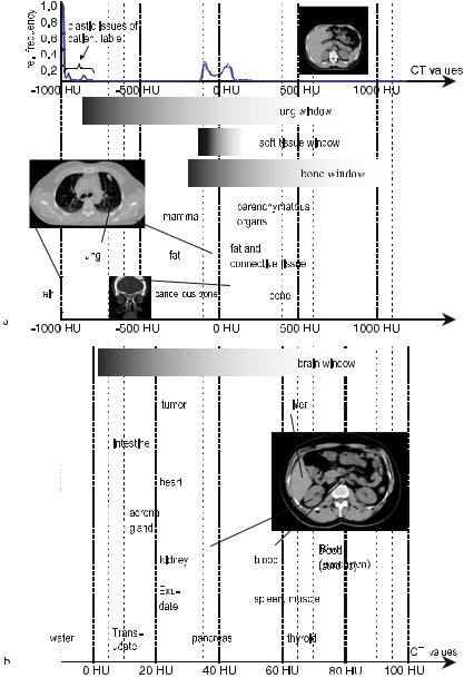
							10.3 Data Representation

Fig. . . Comparison of the di erentiability of tissue when using a soft tissue window (a: WL = + HU, WW = HU), a bone window (b: WL = + HU, WW = , HU), and a lung or pleura window (c: WL = − HU, WW = , HU); data courtesy of Ruhlmann

possible to visualize density di erences between the white and gray matter of the brain. However, it is not possible to assess the calvarium of the skull at the same time, since all CT values larger than – HU are again mapped appearing equally white. For this purpose, one has to select the bone window to be able to di erentiate the higher CT values representing the cranial bone. The bone window representations in Fig. . b and d even allow the spongiosa structure of the cranial bone to be identiﬁed.

10.3.3

Three-Dimensional Representation

Figure . b and c provides images of the volume rendering technique. This method assigns a physical light reﬂection and scattering value to each voxel (spatial pixel). The computer is then used to light up this data fog with a virtual light source and to model the optical impression artiﬁcially. To do so a real reﬂection and scattering of light is simulated.

If bones, organs or contrast media-enhanced vessels are assigned to di erent optical properties, interesting insights into the pathological status of the patient can be gained (cf. Figs. . b–c and . f). In a post-processing step, certain tissue types can be suppressed. In Fig. . d for example, bone is eliminated by a special bone removal technique for better visualization of the vessel tree.

10 Image Quality and Artifacts







Fig. . . Di erentiability of tissue when using a brain window (a: WL = HU,
WW = HU) and a bone window (b: WL =		HU, WW = , HU). T he frequency+
distribution indicates how the brain window	has been selected); data courtesy of Ruhlmann
distribution indicates how the brain window		+

An alternative to volume rendering is surface rendering, as illustrated in Fig. . . The individual shades of gray of the layers (images) in the data stack represent the degree of physical attenuation of the X-ray beam. In a clinical context, deviations from the normal distribution of these values may indicate pathological changes in the patient.

10.3 Data Representation

Fig. . . Angiographic image acquisition with CT (CTA): a Maximum-Intensity Projection (MIP), b volume rendering, c zoom into the knee and visualization from the back, and d virtual bone elimination with the bone removal technique (courtesy of Philips Medical Systems)

Fig. . . Three-dimensional representation of the abdomen. a Coronal reformatting, b–e volume and surface rendering, c–e virtual endoscopy of the intestine together with the representation of the virtual endoscopy trajectory, and e virtually opened intestine in cylinder coordinates (courtesy of Philips Medical Systems)

10 Image Quality and Artifacts

During visualization, it is possible to visualize certain ranges of values and to selectively suppress others. If the viewer chooses a constant gray value, i.e., a threshold, all spatial points with this value may be displayed in space as an iso-surface. This surface is approximated by triangles using a technique called triangulation. Then the mosaic of triangles is again lit and displayed by the virtual method described above. The larger the chosen number of mosaic pieces for the reconstruction of the surface, the more lifelike the result.

In addition to the three-dimensional representation of organs or bone surfaces, which may be interactively rotated on the computer screen, an interior view of hollow organs and airways of contrast-enhanced vessels can be produced. In this way, virtual rides into the body – for example into the bronchial tubes or the intestine – can be visualized. In Fig. . e, a virtual insight into the human intestine is given. The value of such a three-dimensional diagnostic approach lies in the data reduction otherwise being inherent in the hundreds of single slices.

10.4

Some Applications in Medicine

In the ﬁnal section of this chapter, the broad variety of clinical applications of modern CT imaging is summarized by means of some examples. In Fig. . , four typical applications are given. Important ﬁelds of application are summarized in the following:

•Brain perfusion: The blood ﬂow in the brain (cerebral blood ﬂow – CBF), blood volume in the brain (cerebral blood volume – CBV), mean transit time (MTT), and peak time of the bolus maximum (time to peak – TTP) are acquired and displayed as colored overlay onto the relevant CT slices. In this way, colored maps of tissue vitality give indications of an acute or chronic infarct (cf. Fig. . a).

•Liver perfusion: Arterial and portal measurements of perfusion in liver studies.

•Tumor perfusion: Characterization of known lesions via their perfusion.

•Lung measurement: Diagnostics of lung emphysema (cf. Fig. . b); automatic detection of lung nodules.

•Calcium scoring: Quantiﬁcation of coronary calciﬁcation.

•Vessel analysis (CTA): Visualization of vessel trees (cf. Fig. . c); analysis of stenoses and aneurysms; planning of stents.

•Cardio CT: Identiﬁcation and quantiﬁcation of stenoses; planning of stents and visualization of implanted stents (cf. Fig. . d).

•Virtual endoscopy: Three-dimensional CT data as a basis for anatomical interior views of hollow organs (cf. Fig. . e) and contrast-enhanced vessel trees.

•Trauma: Fast imaging of the entire body for diagnostics of accident injuries.

•Dental planning: Three-dimensional reconstruction and slices through the maxilla and mandible as a planning basis for the implantation of prostheses for the oral surgeon.

10.4 Some Applications in Medicine

Fig. . . a Perfusion measurement for stroke patients, b visualization of lung emphysema, c CT angiography of the cranial vessels, and d imaging of a coronary stent (courtesy of Philips Medical Systems)

10 Image Quality and Artifacts

•Planning of radiotherapy: Three-dimensional CT reconstruction as a basis for dose planning in the radiation therapy of tumors.

•Image-guided surgery: Three-dimensional CT reconstruction as a basis for the planning and navigation of surgical interventions.

•Interventional imaging: Visualization of a surgical instrument tip during a biopsy.

In particular, the perfusion measurements show that today’s CT is on the upswing toward becoming a functional modality. This technique allows the blood ﬂow to be measured after contrast media injection into di erent organs.

<<< < Предыдущая 1 2 3 45 / 75 6 7 > Следующая >>>

Соседние файлы в предмете [НЕСОРТИРОВАННОЕ]

#
25.04.201979.36 Кб1Boiler_and_reactor_building_Unit4.doc
#
29.05.201519.47 Кб31Brass.docx
#
29.05.201526.89 Кб22Buddizm.docx
#
29.05.20151.2 Mб34Bukhgaltersky_uchet_UP_2012.doc
#
29.05.20156.06 Mб3103BusinessEnglish_Nikolaenko.pdf
#
29.05.201515.29 Mб42Buzug_Computed_tomography_From_photon_stat.pdf
#
29.05.2015403.08 Кб23BZhD_otvety-1.pdf
#
17.09.2019822.27 Кб9bzhd_otvety.doc
#
23.11.2019302.59 Кб6b_12101809_t_k_r_fizika.doc
#
25.08.20191.49 Mб69C2.doc
#
29.05.20151.42 Mб27CFZ_TREBOVANIYa.doc