


4Fundamentals of Signal Processing
Contents |
|
|
4.1 |
Introduction . . . . . . . . . . . . . . . . . . . . . . . . . . . . . . . . . . . . . . . . . . . . . . . . . . . . . . . |
102 |
4.2 |
Signals . . . . . . . . . . . . . . . . . . . . . . . . . . . . . . . . . . . . . . . . . . . . . . . . . . . . . . . . . . . . |
102 |
4.3 |
Fundamental Signals . . . . . . . . . . . . . . . . . . . . . . . . . . . . . . . . . . . . . . . . . . . . . . . . . |
102 |
4.4 |
Systems . . . . . . . . . . . . . . . . . . . . . . . . . . . . . . . . . . . . . . . . . . . . . . . . . . . . . . . . . . . |
104 |
4.5 |
Signal Transmission . . . . . . . . . . . . . . . . . . . . . . . . . . . . . . . . . . . . . . . . . . . . . . . . . . |
106 |
4.6 |
Dirac’s Delta Distribution . . . . . . . . . . . . . . . . . . . . . . . . . . . . . . . . . . . . . . . . . . . . . . |
109 |
4.7 |
Dirac Comb . . . . . . . . . . . . . . . . . . . . . . . . . . . . . . . . . . . . . . . . . . . . . . . . . . . . . . . . |
112 |
4.8 |
Impulse Response . . . . . . . . . . . . . . . . . . . . . . . . . . . . . . . . . . . . . . . . . . . . . . . . . . . |
115 |
4.9 |
Transfer Function . . . . . . . . . . . . . . . . . . . . . . . . . . . . . . . . . . . . . . . . . . . . . . . . . . . . |
116 |
4.10 |
Fourier Transform . . . . . . . . . . . . . . . . . . . . . . . . . . . . . . . . . . . . . . . . . . . . . . . . . . . |
118 |
4.11 |
Convolution Theorem . . . . . . . . . . . . . . . . . . . . . . . . . . . . . . . . . . . . . . . . . . . . . . . . |
124 |
4.12 |
Rayleigh’s Theorem . . . . . . . . . . . . . . . . . . . . . . . . . . . . . . . . . . . . . . . . . . . . . . . . . . . |
125 |
4.13 |
Power Theorem . . . . . . . . . . . . . . . . . . . . . . . . . . . . . . . . . . . . . . . . . . . . . . . . . . . . . |
125 |
4.14 |
Filtering in the Frequency Domain . . . . . . . . . . . . . . . . . . . . . . . . . . . . . . . . . . . . . . . |
126 |
4.15 |
Hankel Transform . . . . . . . . . . . . . . . . . . . . . . . . . . . . . . . . . . . . . . . . . . . . . . . . . . . |
128 |
4.16 |
Abel Transform . . . . . . . . . . . . . . . . . . . . . . . . . . . . . . . . . . . . . . . . . . . . . . . . . . . . . |
132 |
4.17 |
Hilbert Transform . . . . . . . . . . . . . . . . . . . . . . . . . . . . . . . . . . . . . . . . . . . . . . . . . . . |
133 |
4.18 |
Sampling Theorem and Nyquist Criterion . . . . . . . . . . . . . . . . . . . . . . . . . . . . . . . . . . |
135 |
4.19 |
Wiener–Khintchine Theorem . . . . . . . . . . . . . . . . . . . . . . . . . . . . . . . . . . . . . . . . . . . |
141 |
4.20 |
Fourier Transform of Discrete Signals . . . . . . . . . . . . . . . . . . . . . . . . . . . . . . . . . . . . . |
144 |
4.21 |
Finite Discrete Fourier Transform . . . . . . . . . . . . . . . . . . . . . . . . . . . . . . . . . . . . . . . . |
145 |
4.22 |
z-Transform . . . . . . . . . . . . . . . . . . . . . . . . . . . . . . . . . . . . . . . . . . . . . . . . . . . . . . . . |
147 |
4.23 |
Chirp z-Transform . . . . . . . . . . . . . . . . . . . . . . . . . . . . . . . . . . . . . . . . . . . . . . . . . . . |
148 |
4 Fundamentals of Signal Processing
4.1 Introduction
The entire theory of the continuously developing area of signal processing is beyond the scope of this chapter. In this chapter, only the principal methods of signal processing that are important for computed tomography (CT) will be described. In contrast to most essays on signal processing, descriptions of the signals in the spatial domain will be used – since it is in this form that signals are present in X-ray and CT imaging modalities.
4.2 Signals
The signals being considered here are one-dimensional spatial signals: s(x) – for instance from a detector array of a CT scanner, or two-dimensional images: f (x, y) – e.g., one slice of a D CT image. The signals are either continuous or, after sampling, discrete functions of one or more variables.
4.3
Fundamental Signals
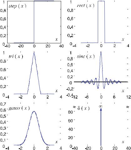
In signal processing, some fundamental signals are extraordinary in the sense that the deformation of a signal throughout its transmission enables conclusions to be drawn about the system itself. These fundamental signals are given in ( . ) to ( . ), as well as in Fig. . .
|
|
|
|
|
( ) = & |
x |
: |
|
|
|
|
|
|
|
|||||
Heaviside step function |
step |
|
x |
|
|
|
|
|
|
|
|
|
( . ) |
||||||
|
|
|
|
otherwise |
|
|
|||||||||||||
|
|
|
|
( |
|
) = & |
|
|
|
||||||||||
|
|
|
|
|
|
x |
|
|
|
|
|
|
|||||||
Rectangular function |
rect |
|
x |
|
|
|
|
|
|
|
|
|
|
( . ) |
|||||
|
|
|
|
otherwise |
|
|
|||||||||||||
|
|
( ) = & − |
|
|
|
|
|||||||||||||
|
|
x |
|
x |
|
|
|
|
|
||||||||||
Triangle function |
tri |
|
x |
|
|
|
|
|
|
|
|
|
|
|
( . ) |
||||
|
|
|
|
|
|
|
|
otherwise |
|||||||||||
|
( |
|
) |
|
|
|
|
|
|||||||||||
Sinc function |
|
|
( ) = |
|
sin |
( |
πx |
) |
|
||||||||||
si |
|
x |
|
|
|
sinc |
x |
|
|
|
|
|
|
|
|
|
( . ) |
||
|
|
|
|
|
|
|
|
|
|
|
|
|
πx |
|
|
|
|||
|
|
|
gauss(x) = |
|
|
|
|
|
|
|
|
|
|
||||||
Gaussian function |
|
|
6 |
|
e−x |
|
|
|
( . ) |
||||||||||
|
|
π |
|
|
|
||||||||||||||
|
|
|
|
4.3 Fundamental Signals |
|
||
|
|
|
|
|
|
|
|
|
|
|
|
|
|
|
|
|
|
|
|
|
|
|
|
|
|
|
|
|
|
|
|
|
|
|
|
|
|
|
|
|
|
|
|
|
|
|
|
|
|
|
|
|
|
|
|
|
|
|
|
|
|
|
|
|
|
|
|
|
|
|
|
|
|
|
|
|
|
|
|
Fig. . . Illustration of some of the fundamental functions of signal processing. By analyzing the changes that these signals experience within linear and complex systems, conclusions can be drawn about the systems themselves. Dirac’s delta “function” is of particular importance. It is connected to the “impulse response” of the system, which will be used frequently in later chapters. Due to the importance of the delta impulse, which is actually a distribution, this “function” is described in detail in Sects. . – .
Delta distribution |
|
|
|
+ |
( |
x |
) |
δ |
( |
x |
− |
x |
) |
dx |
= |
f |
( |
x |
) |
( . ) |
||
|
|
|
− |
|||||||||||||||||||
|
|
|
∫ f |
|
|
|
|
|
|
|
|
|||||||||||
|
|
|
|
|
|
|
or formally, |
|
|
|
|
|
|
|
||||||||
|
( − ) = & |
x |
= |
x |
|
|
|
|
|
|
|
+ |
|
( − ) = |
|
|||||||
|
|
|
|
|
|
|
− |
|
|
|
||||||||||||
|
|
|
|
|
|
|
|
|
|
|
∫ δ x |
|
|
|
|
|
|
|||||
δ x x |
|
x |
8 x |
|
|
and |
|
|
x |
dx . |
( . ) |
|||||||||||
4 Fundamentals of Signal Processing
4.4 Systems
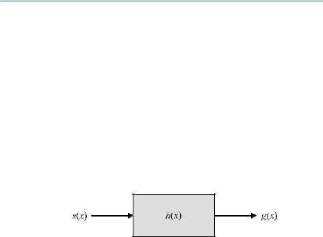
Systems process signals. In particular, one refers to a “transmission system,” and describes it by an output signal, g(x), corresponding to a specific input signal, s(x). The transformation equation can be formally written as
g x, |
(y |
) = L f |
|
(x,) |
|
( . ) |
|||
g |
x |
s |
|
x |
) |
|
|||
( |
|
) = L |
|
( |
y |
. |
( . ) |
||
|
|
|
|
|
|
|
|||
A transformation can also be represented schematically by a block diagram, as shown in Fig. . .
In general, transmission systems are described in terms of their attributes linearity, spatial invariance, shift-invariance, causality, and stability. T hese properties are briefly introduced in the following sections.
Fig. . . Schematic block diagram illustrating the signal transmission. h(x) is called the impulse response
4.4.1 Linearity
A system is linear if, for all ai ; C,
L& ai si (x)' = ai gi (x) , |
( . ) |
|||
|
i |
i |
|
|
or, in the two-dimensional case, |
|
|
|
|
L& i |
ai fi (x, y)' = i |
ai gi (x, y) . |
( . ) |
|
An example of a linear transmission system in image processing is an edge filter for horizontal edges, which, in its simplest form, can be described by
L fi (x, y) fi (x, y) − fi (x, y + ) = gi (x, y) . |
( . ) |
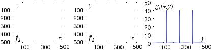
The edge filter detects gray-value changes in images, like those provided in Fig. . . The two images on the left of Fig. . contain horizontal gray-value edges with a step
|
|
|
|
|
4.4 Systems |
|
|
|
|
|
|
|
|
|
|
|
|
|
|
|
|
|
|
|
|
|
|
|
|
|
|
|
|
|
|
|
|
|
|
|
|
|
|
|
|
|
|
Fig. . . Due to scale values, but The response, gi
the linearity of the edge filter, two images that di er in their absolute graywhich have horizontal edges of the same step size, yield the same response. (•, y), is illustrated on the right as a vertical profile
size of units of gray-scale intensity at each step. The gray-value level in the middle image is units higher than in the image on the left. It is important that the edge filter gives the same response to the gray-value change in the lef t image
f x, y |
|
|
f x, y |
|
|
( . ) |
change in the central image |
|
|
||||
as it does to the gray-value( |
) = |
|
( |
+ ) = |
|
|
f (x, y) = f (x, y + ) = . |
( . ) |
|||||
The response of the edge filter is displayed as a profile in Fig. . (right). The horizontal edges yield to the same response for both images.
4.4.2
Position or Translation Invariance
A transmission system is said to be position invariant, or alternatively shift invariant if, for arbitrary x , y
|
s x x |
g x x |
( . ) |
or, in the two-dimensional |
case |
) = ( − ) |
|
L ( − |
|
||
L f (x − x , y − y ) = g(x − x , y − y ) . |
( . ) |
||
Although ( . ) and ( . ) look like self-evident properties, one cannot assume that real systems are position or translation invariant. For example, image distortion can violate these properties. A common acronym for linear translation invariant systems is “LTI systems.”
4.4.3
Isotropy and Rotation Invariance
During the transmission of generalized images with two or more dimensions, their shape does not change in the presence of isotropy or rotation invariance. The example of an edge filter provided in Fig. . is only an isotropic system if the result of the filter is independent of the orientation of the edge and always yields the same response.
|
4 Fundamentals of Signal Processing |
4.4.4 Causality
In the case of causal transmission systems, the output signal is not known prior to the input signal. This is always true for real online systems. In system theory, noncausal systems are likely to be used for calculations, due to their straightforward mathematical treatment (Lüke ). Strictly speaking, the term “causality” is only applicable in the case of time signals. Generally, in image processing applications, an image is present in its entirety and signal processing takes place with respect to its spatial coordinates (Werner ).
4.4.5 Stability
A system is said to be “amplitude-stable” if it responds to an amplitude-bounded input signal with an amplitude-bounded output signal. Those systems are also called “BIBO” systems (bounded input–bounded output). In engineering, unstable systems can be problematic due to, for instance, the overflow of a number format that can cause feedback processes in a software module to be controlled by absurd results.
4.5
Signal Transmission
To analyze transmission systems, the fundamental signals ( . ) to ( . ) are used because their modulation allows conclusions to be made quite easily about the system. The concept of the utilization of fundamental signals will be explained in the following paragraphs. One of these signals is the normalized rectangular function
|
|
s (x) = |
|
rect |
x |
, |
( . ) |
|
|
X |
X |
||||
with width X and height |
X . This function is based on the fundamental rectan- |
||||||
gular signal ( . ). |
|
|
|
|
|
|
|
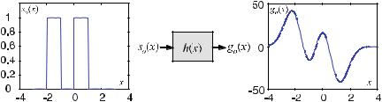
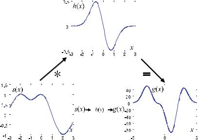
Figure . shows how a signal consisting of two consecutive normalized rectangular signals is deformed by a linear transmission system. The deformation is
Fig. . . Transformation via transmission of the input signal, s (x), consisting of two consecutive rectangular signals. The linear transmission system is described by h(x), which is called the “impulse response” of the system
|
|
|
|
|
|
|
|
|
4.5 Signal Transmission |
|
|||
given by the system’s specific property, which is described by what is called the “im- |
|
||||||||||||
pulse response,” h |
( |
x |
) |
. The impulse response of a system will be described in detail |
|
||||||||
in |
Sect. . . |
|
|
|
|
|
|
|
|
|
|
||
|
To aid the understanding of sampling, and therefore digitization of an analog |
|
|||||||||||
signal, the step function based on the rectangular function is used as an approx- |
|
||||||||||||
imation of an arbitrary signal, s |
x |
. Therefor, the so-called gate property of the |
|
||||||||||
rectangular function is used. |
Figure . shows this behavior where a segment of |
|
|||||||||||
|
( |
) |
( |
|
) |
|
|
||||||
a waveform of finite length is selected. The analog signal, s |
x |
, is approximated at |
|
||||||||||
the position nXo by the rectangular function |
|
|
|
||||||||||
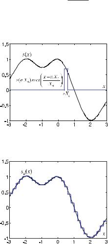
re(x) = s(nX )rect x − nX ,
X
where s(nX ) denotes the height of the signal, s(x), at the position nX and, the rect function is responsible for the gating.
Fig. . . Gate property of the rectangular function. The analog signal, s(x), is approximated by the rectangular function having width X and height s(nX ) at the position nX
Fig. . . Approximation of a signal by a step function. The smaller the width of consecutive rectangles, the more accurately the step function approximates the original analog signal
|
4 Fundamentals of Signal Processing |
|
|
|
|
|
|
|
|
|
|
|
|
|
|
||||||||
|
For the approximation of the entire signal, s |
|
x |
) |
, rectangular functions are com- |
||||||||||||||||||
|
bined resulting in the “step function,” as follows( |
|
|
|
|
|
|
|
|
|
|||||||||||||
|
s |
|
x |
|
sa |
|
x |
|
|
|
nX |
|
rect |
|
x |
nX |
|
|
. |
( . ) |
|||
|
( |
) |
( |
) = |
n =− s |
( |
) |
|
|
−X |
|
||||||||||||
|
|
|
|
|
|
|
|
|
|
|
|
|
|
|
|
||||||||
Figure . illustrates how an analog signal is approximated discretely by a sequence of rectangles, which are normalized accordingly.
The smaller the width of each rectangle, the more accurately the step function approximates the analog signal. Using the definition of the normalized rectangular function ( . ) gives
|
|
|
|
|
|
|
|
|
sa(x) = n =− s(nX )s (x − nX )X . |
( . ) |
|||||
If the transmission system is linear and positionor translation-invariant, the trans- |
|||||||
mitted signal satisfies |
|
|
|
|
|
|
|
g x |
ga x |
|
|
s nX g x |
nX X . |
( . ) |
|
|
n =− |
||||||
( ) ( ) = |
|
( |
) ( − |
) |
|
||
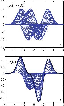
Fig. . . Approximation of the output signal by superposition of individual system responses. The bottom image shows the result of the summing, as well as the convergence of the sum of the respective system responses of the particular fundamental rectangular signals – shown in the top image – toward the overall system response (cf. Fig. . )
4.6 Dirac’s Delta Distribution |
|
In this way, the approximated output signal results from the superposition of the system response to the di erently weighted rectangular impulses. Figure . shows the individual system responses to the rectangular impulses and the result of the summation. At the top of Fig. . , the individual responses to all rectangles of the step function from Fig. . are shown.
The description of an entire transmission by a summation of individual responses, as given by ( . ), is a typical characteristic of linear systems. This is also to be seen in the theory of linear di erential equations, where the sum of weighted, individual results represents the general result. At the bottom of Fig. . , it can be seen how the sum of the individually transmitted fundamental signals converges with the overall result (cf. also Fig. . ).
4.6
Dirac’s Delta Distribution
The signal s(x), as introduced in the previous paragraph, is more accurately approximated by using a normalized rectangular impulse of smaller width X in ( . ), while the area of the impulse remains unity in its normalized representation. Hence, the narrower the impulse, the larger the amplitude, X .
The limit
δ(x) = |
lim |
|
|
x |
|
|
|
rect X |
( . ) |
||||
X X |
||||||
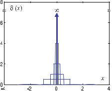
defines Dirac’s delta impulse, or more precisely the δ-distribution, which was introduced above as an elementary “function” in ( . ) and ( . ). Figure . shows schematically how ( . ) tends toward the limit. The limit gives a “spike” impulse of infinite height and vanishing width.
Fig. . . Tendency toward the limit from a normalized rectangular impulse to a spike impulse of infinite height. The resulting δ-distribution is of great importance in the theory of sampling of analog signals
|
4 Fundamentals of Signal Processing |
It should be noted that alternative limit representations of the δ-distribution exist, such as
|
δ(x) = |
|
lim |
|
|
|
− x |
|
|
|||||
|
|
|
|
|
X |
|
||||||||
|
|
|
|
|
|
|||||||||
or |
X X e |
|
) |
|
|
( . ) |
||||||||
|
|
( |
|
) = |
|
|
sin |
( |
πεx |
|
|
|
||
|
δ |
|
x |
|
|
lim |
|
|
|
|
|
|
. |
( . ) |
|
|
|
|
|
ε |
|
|
πx |
|
|
|
|
|
|
These will be used later on (cf. ( . )). Further representations can be found in Barrett and Swindell ( ).
The application of the limit in ( . ) means that the location of the gating must be replaced by
nX ξ
and the width of the gating by
Xo dξ .
In this way one obtains the important property
+
s(x) = ∫ s(ξ)δ(x − ξ)dξ
−
= s(x) > δ(x) ,
or for the two-dimensional case of an image
f (x, y) = |
+ + |
∫ ∫ f (ξ, η)δ(x − ξ, y − η)dξ dη |
− −
= f (x, y) > δ(x, y) ,
( . )
( . )
( . )
( . )
which is a so-called convolution. ( . ) is symmetric with respect to the permutation of the integration variables, such that
|
|
( |
|
|
+ |
( |
|
) |
|
( |
|
− |
|
) |
|
|
||
|
|
|
|
) =− |
|
|
|
|
|
|
|
|||||||
|
s |
|
|
ξ |
∫ |
s |
|
x |
|
δ |
|
x |
|
|
ξ |
|
dx |
( . ) |
is satisfied. By simple substitution, it holds that |
|
|
|
|
|
|||||||||||||
|
(− |
|
+ |
( |
|
− |
|
) |
|
( |
|
) |
|
|
||||
|
|
) =− |
|
|
|
|
|
|
|
|||||||||
s |
|
|
ξ |
∫ |
s |
|
y |
|
|
ξ |
|
δ |
|
y |
|
dy . |
( . ) |
|
( . ) is called the “sifting property” of the δ-distribution.
Two further properties are mentioned explicitly here, as they will be needed in the following chapters. First of all, the scaling property for δ(ax), with a 8 , should be analyzed. The familiar interpretation as a stretching of the function is not

4.6 Dirac’s Delta Distribution |
|
applicable in the case of an impulse of width zero. However, from the definition in ( . ), it follows that the normalization of the integral is given as
+ |
|
∫ δ(x)dx = , |
( . ) |
−
which raises the question once again, of what meaning δ(ax) has as an integrand. To address this question, consider the simple substitution y = ax, resulting in
+ |
( |
|
) |
|
= a |
+ |
( |
|
) |
|
= a |
+ |
( |
|
) |
|
|
|||
− |
|
|
− |
|
|
|
− |
|
|
|
||||||||||
∫ δ |
|
ax |
|
dx |
|
|
∫ |
δ |
|
y |
|
dy |
|
|
∫ δ |
|
x |
|
dx . |
( . ) |
|
|
|
|
|
|
|
|
|
|
|||||||||||
Since the δ-distribution is symmetric, δ(−x) = δ(x), and therefore in general,
|
|
δ(ax) = a δ(x) . |
( . ) |
Occasionally, the argument of the δ-distribution itself is a complicated function, g(x), of the spatial variable x. This further property, which will be required inSect. . for the calculation of the properties of the simple backprojection, is briefly described here.
If g(x) has a single root at x = x , it is evident that δ(g(x)) vanishes everywhere except for the infinitesimal neighborhood of x = x . Taking the Taylor expansion of g(x) in the region of the root x gives
δ(g(x)) = δ g(x ) + (x − x ) dx ?x . |
( . ) |
|
|
dg |
|
Higher order terms of the Taylor expansion are not required, as the neighborhood around x is arbitrarily small. Since g(x ) = is satisfied, it immediately follows that
( ( )) = ? dx @x |
? |
|
|
||
|
x |
x |
|
||
δ g x |
δ( dg− |
|
) |
. |
( . ) |
In this way, one can exploit the scaling property, ( . ), of the δ-distribution. If
the function g(x) has more than one root, |
( . ) can be generalized by |
|
||||||||
δ x |
xi |
|
||||||||
|
( |
|
( |
|
)) = |
? dx |
@xi ? |
|
||
δ |
|
g |
|
x |
i |
( |
dg− ) |
. |
( . ) |
|
|
|
|
|
|
|
|
|
|
||
The fundamental properties of the δ-distribution are given in Table . . Additional properties can be found, for example, in Messiah ( ), Klingen ( ) or in Bracewell ( ).
( . ) to ( . ) imply that one is allowed to replace the left side with the expression on the right side, if it occurs as an integrand of an integral over x.
|
4 Fundamentals of Signal Processing |
|
|
|
|
||||
|
Table . . Fundamental properties of the δ-distribution according to Messiah ( ), Klingel |
||||||||
|
( ), and Bracewell ( ) |
|
|
|
|
|
|
|
|
|
|
|
|
|
|
|
|
|
|
|
|
|
|
δ(x) = δ(−x) |
|
( . ) |
|||
|
aδ(x) + bδ(x) = (a + b)δ(x) |
( . ) |
|||||||
|
δ(g(x)) = i |
g (xi ) − δ(x − xi ) |
( . ) |
||||||
|
with xi being single roots of g(x). Especially for g(x) = ax it holds that |
|
|||||||
|
|
|
|
|
|
|
|
|
|
|
δ(ax) = a δ(x) , if a |
( . ) |
|||||||
|
|
|
|
|
xδ(x) = |
|
( . ) |
||
|
f (x)δ(x − a) = f (a)δ(x − a) |
( . ) |
|||||||
|
∫ δ(x − y)δ(y − a)dy = δ(x − a) |
( . ) |
|||||||
|
δ(x − a) δ(x − b) = δ(x − a − b) |
( . ) |
|||||||
|
|
d |
|
step(x) = δ(x) |
( . ) |
||||
|
|
dx |
|||||||
|
δ(x − a)δ(x − b) = |
if a b |
( . ) |
||||||
|
|
( |
|
) = |
|
+ |
|
|
|
|
δ |
x |
∫ eikx dk |
( . ) |
|||||
|
π |
||||||||
|
|
|
− |
|
|
||||
|
|
|
|
|
|
|
|
|
|
4.7
Dirac Comb
The sift property ( . ) of the δ-distribution is used for sampling an analog signal. T his is to be done using the so-called Dirac comb
( |
|
) = |
+ |
( |
) ( |
|
− |
|
) = |
( |
|
) |
+ |
( |
|
− |
|
) |
|
|
x |
|
x |
nX |
x |
|
x |
nX |
. |
( . ) |
|||||||||||
sa |
|
n =− |
s |
nX δ |
|
|
s |
|
n =− |
δ |
|
|
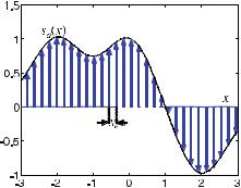
Figure . shows how a function, s(x), is sampled by the Dirac comb. Unlike the step function ( . ), which approximates the analog signal, the periodic, needleshaped δ-distribution now measures the analog signal precisely at discrete points.
The expression δ(x)δ(x) is not defined.
4.7 Dirac Comb |
|
Fig. . . The process of sampling an analog signal using a Dirac comb. Contrary to the concept of the step function in Fig. . , here the signal s(x) is sampled at equidistant discrete points with intervals of Xo. The comb is represented by arrows for visualization purposes only. Mathematically, the height of Dirac’s delta impulse does not vary; rather, the sampled values are the weights of Dirac’s delta impulse train
Due to the appearance of the impulse train, Bracewell ( ) denoted the Dirac comb by the Cyrillic letter Ш (pronounced “shah”), which is therefore shown by
where |
sa(x) = s(x)Ш(x) |
|
|
( . ) |
|||||||
|
( |
) = |
+ |
|
( |
|
− |
|
) |
|
|
|
|
δ |
x |
nX |
. |
( . ) |
|||||
|
Ш x |
|
|
|
|
|
|||||
n =−
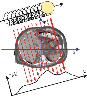
For CT the sift property has to be expressed two-dimensionally. In two dimensions, it is possible to construct δ-lines from spike impulses, δ(x, y), which can be considered as a contiguous “lining-up” of δ-spike impulses. Figure . shows how an anatomical object (in this case a section through the abdomen) is sampled along parallel lines.
Integration of the attenuation values, which are given by the spatial distribution f (x, y), can be written as a one-dimensional integral in a Cartesian coordinate system, (ξ, η), which is rotated by angle γ with respect to the (x, y) patient frame
|
( |
|
+ |
|
( |
( |
) − |
( |
) |
|
( |
|
) + |
|
( |
|
)) |
|
|
pγ |
|
) =− |
|
|
|
|
|
|
|
||||||||||
|
ξ |
∫ |
f |
|
ξ cos γ |
|
η sin γ |
|
, ξ sin |
|
γ |
|
η cos |
|
γ |
|
dη . |
( . ) |
The η-axis is aligned with the direction of a given projection, i.e., the lines along which attenuation information is summed up by the integration. In the particular case of CT, this is the direction of the X-rays.
|
4 Fundamentals of Signal Processing |
||
|
|
|
|
|
|
|
|
Fig. . . Two-dimensional spatial sampling of an object along parallel lines in computed tomography. The response, pγ (ξ), measures the sum of all attenuation values along the X- ray lines of the current projection angle, γ. The signal of interest is the spatial distribution of the attenuation values, f (x, y)
( . ) can also be described as a convolution with a δ-line, where the sift property of the δ-distribution is employed, giving
pγ (ξ) = f (x, y) > δ(L) = ∫∫ f (x, y)δ((x, y) − L)dx dy ( . )
(x, y) R
or alternatively
f > δ(L) = ∫ f (r)δ(r − L)dr = ∫ f (r)dr. ( . )
r L
In this way, one obtains the projection of all values on the path of the X-ray along the line L through the object onto the ξ-axis.

4.8 Impulse Response |
|
4.8
Impulse Response
The way in which physical objects and systems are examined always comes down to the same principle. One tries to excite the system and waits for the response. If one has a detailed knowledge of the excitation, many properties of the system can be determined well. An exceptionally simple excitation of a system can be achieved by Dirac’s delta impulse.
The response of a transmission system to the delta distribution, or δ-impulse, is given by
|
( |
|
+ |
( |
|
) |
|
( |
|
− |
|
) |
|
|
|
|
) =− |
|
|
|
|
|
|
||||||
s |
|
ξ |
∫ s |
|
x |
|
δ |
|
ξ |
|
x |
|
dx , |
( . ) |
which is essentially exploiting the sift property. In the case of a linear transmission system
it reads |
|
|
|
|
|
|
g(x) = L s(x) , |
|
|
|
|
|
|
( . ) |
||||||||
|
( |
|
) = |
|
( |
|
) > |
|
( |
|
+ |
( |
|
) |
|
( |
|
− |
|
) |
|
|
|
|
|
|
|
|
) =− |
|
|
|
|
|
|
||||||||||
g |
|
x |
|
s |
|
x |
|
h |
|
x |
∫ s |
|
ξ |
|
h |
|
x |
|
ξ |
|
dξ , |
( . ) |
where h(x) denotes the already mentioned impulse response.
Figure . gives an example of the transmission of a signal s(x) via the impulse response
|
x |
|
|
||
h(x) = − |
6 |
|
e−x |
. |
( . ) |
π |
|||||
Note that the arbitrarily chosen impulse response function ( . ) is the same as the
one used in |
|
Sect. . . |
|
|
|
|
|
|
|
|
|
|
|
|
|
|
|
|||
The |
response given by ( . ) can be extended for two-dimensional systems by |
|||||||||||||||||||
|
|
|
|
|
|
|
|
|
|
|
|
|
|
|
|
|
|
|
|
|
|
|
|
|
( |
|
+ + |
|
( |
|
) |
|
( |
|
− |
|
− |
|
) |
|
|
|
|
|
|
|
) =− − |
|
|
|
|
|
|
|
|
|||||||
|
|
|
g |
|
x, y |
∫ ∫ |
f |
|
ξ, η |
|
h |
|
x |
|
ξ, y |
|
η |
|
dξ dη. |
( . ) |
( . ) describes the fundamental equation of system theory for imaging systems. The response of the system is called the point-spread function. It follows that a linear
|
4 Fundamentals of Signal Processing |
||||||||
|
|
|
|
|
|
|
|
|
|
|
|
|
|
|
|
|
|
|
|
|
|
|
|
|
|
|
|
|
|
|
|
|
|
|
|
|
|
|
|
|
|
|
|
|
|
|
|
|
|
|
|
|
|
|
|
|
|
|
|
Fig. . . Transmission of a signal. The transmitted signal is given by the convolution of the signal s(x) with the system’s impulse response h(x)
transmission system with a point-spread function, h |
( |
x, y |
) |
, responds to an input |
||||||||||||||
image, f |
x, y |
|
, with an output image |
|
( |
|
) > |
|
( |
|
|
|
|
|||||
( |
|
) |
g |
( |
x, y |
) = |
f |
x, y |
h |
x, y |
) |
, |
|
( . ) |
||||
|
|
|
|
|
|
|
|
|
||||||||||
where ( . ) is the standard notation used to abbreviate ( . ).
4.9
Transfer Function
The question of how to determine the impulse response of a system still remains. For this purpose, specific functions are applied to the system of interest. Consider the following eigenvalue problem
Lσ = Hσ , |
( . ) |
where L is again a linear operator, σ is a so-called eigenfunction of the system and H denotes a constant, i.e., the system’s eigenvalue. Let the linear operation L be given by
|
|
σ |
|
σ |
h x . |
( . ) |
The eigenfunctions can be |
described by |
> ( ) |
|
|||
L |
|
|
|
|
||
σ(x) = ei πux = cos( πux) + i sin( πux), |
( . ) |
|||||

4.9 Transfer Function |
|
where u is the spatial frequency of the system. The application of the linear operator
to the eigenfunction gives
g(x) = σ(x) > h(x)
|
|
|
+ |
|
( |
|
) |
|
|
|
|
|
|
|
|
|
∫ |
h |
ξ |
ei πu(x−ξ)dξ |
|
||||||
|
=− |
|
|
|
|
|
|
( . ) |
|||||
|
|
|
|
|
|
+ |
|
|
|
||||
|
= ei πux ∫ h(ξ)e−i πu ξ dξ . |
|
|||||||||||
Hence, the eigenvalues are given by |
|
|
− |
|
|
|
|
||||||
|
|
|
|
|
|
|
|
|
|
||||
|
( |
|
|
+ |
|
( |
|
) |
|
|
|||
H |
u |
|
∫ |
h |
x |
e−i πux dx . |
( . ) |
||||||
|
|
) =− |
|
|
|
|
|
||||||
( ) on the spatial frequency.
The eigenvalues H u provide the amplitudes and phases of the system that depend
In the case of an image, ( . ) can again be extended so that in the twodimensional domain,
( |
|
+ + |
( |
|
) |
|
|
|
) =− − |
|
|
|
|||
H |
u, v |
∫ ∫ |
h |
x, y |
|
e−i π(ux+v y) dx dy |
( . ) |
is valid, where u denotes the spatial frequency in the frequency in the y direction. If one defines
u = |
|
, |
v = |
|
and kx = |
π |
, |
λx |
λy |
λx |
x direction and v the spatial
ky = |
π |
, |
( . ) |
λy |
the k-space representation of the Fourier transform
( |
|
+ + |
( |
|
) |
|
|
|
) =− − |
|
|
|
|||
H |
kx , ky |
∫ ∫ |
h |
x, y |
|
e−i(kx x+k y y) dx dy |
( . ) |
can be obtained. This equation describes the Fourier transform, whose formal notation in one dimension is often given by
H |
|
|
h |
|
or |
|
h ——— H . |
|
|||
|
Fourier transform must be inverted, resulting in |
||||||||||
As one is interested in h, the= F |
|
|
|
|
A |
• |
|
||||
or |
|
|
|
h = F− H |
|
( . ) |
|||||
|
( |
|
|
+ |
( |
|
) |
|
|
|
|
|
|
) =− |
|
|
|
|
|||||
h |
|
x |
|
∫ |
H |
|
u |
|
ei πux du , |
( . ) |
|
or alternatively for the point-spread function in the two-dimensional case |
|
||||||||||
h(x, y) = |
+ + |
|
|
|
|
|
|
|
|||
∫ ∫ H(u, v)ei π(ux+v y) du dv . |
( . ) |
||||||||||
− −

|
4 Fundamentals of Signal Processing |
|
This means that the transfer function of a system is the Fourier transform of the |
|
corresponding impulse response (Lüke ). Please note, if the k-space notation is |
|
used for the inverse Fourier transform – analog to ( . ) – a normalization factor |
|
of ( π)− must be introduced for each dimension. |
4.10
Fourier Transform
Due to the importance of the Fourier transform not only in the field of signal processing for CT, it is briefly introduced here. In the upcoming chapters, in which the reconstruction mathematics of CT will be considered, the following definition of
a function’s Fourier transform is used. |
|
|
|
|
|
|
|
|
|
|
|
|||||||||
If f x |
|
is a real or complex-valued function of the variable x, then its Fourier |
||||||||||||||||||
transform, if it exists, is the function |
|
|
|
|
|
|
|
|
|
|
|
|||||||||
( |
) |
|
|
|
|
|
|
|
+ |
|
|
|
|
|
|
|
|
|
|
|
|
|
|
|
|
|
|
|
|
|
|
|
|
|
|
|
|
|
|
|
|
|
|
|
( |
|
) = |
π |
|
− |
( |
|
) |
|
F |
|
( |
|
) |
|
|
|
|
|
F |
|
u |
|
α |
|
∫ f |
|
x |
|
e−iαux dx |
|
f |
|
x |
|
, |
( . ) |
|
|
|
|
|
|
|
|
|
|
|
|
|
|||||||||
where α is a constant whose origin is di erent in the field of signal processing from that in other applications. In quantum mechanics, for example, one often chooses the reciprocal of Planck’s constant (normalized by π), which is α = ħ. T hroughout later chapters, the definition α = π is used.
f (x) results from F(u) by inversion of the Fourier transform
|
|
|
|
|
|
|
+ |
|
|
|
|
|
|
|
|
|
|
|
|
|
|
( |
|
) = |
π |
|
− |
( |
|
) |
|
F |
|
|
|
( |
|
) |
|
|
|
f |
|
x |
|
α |
|
∫ F |
|
u |
|
eiαux du |
|
− |
|
F |
|
u |
|
. |
( . ) |
|
|
|
|
|
|
|
|
|
|
|
|
||||||||||
Using this symmetric definition allows us to avoid confusion regarding which normalization term must be written in front of the integral of the transform and its inverse. In more general terms, with f (x , x , x , . . . , xn ) being a function of the n variables x , x , x , . . . , xn , the Fourier transform is defined by
|
|
|
|
|
|
|
α |
|
|
|
n |
+ |
+ |
|
|
|
|
|
|
F |
|
u , . . . , un |
|
|
|
|
|
|
|
∫ . . . |
∫ f |
|
|
x , . . . , xn |
|
e−iα(u x + ... +un xn ) dx . . . dxn |
|||
( |
) = π |
|
|
( |
) |
||||||||||||||
|
|
|
|
|
|
− − |
|
( . ) |
|||||||||||
and its inverse is given by |
|
|
|
|
|
|
|
||||||||||||
|
( |
|
|
|
|
α |
|
|
n |
+ |
+ |
|
|
|
|
|
|||
f |
x , . . . , xn |
|
|
|
|
|
|
∫ . . . ∫ F |
|
u , . . . , un |
|
eiα(u x + ... +un xn ) du . . . dun . |
|||||||
) = π |
|
|
|
( |
) |
||||||||||||||
|
|
|
|
− − |
|
|
( . ) |
||||||||||||
Important properties of the Fourier transform are summarized in Table . .
It very often happens that the forward transform and the inverse transform are of unequal di culty.

|
|
|
|
|
|
|
|
|
|
|
|
|
|
|
|
|
|
|
|
|
|
|
|
|
|
|
|
|
|
|
|
|
|
|
|
4.10 |
Fourier Transform |
|
||
Table . . Important properties of the Fourier transform according to Messiah ( ), Klingel |
|
|||||||||||||||||||||||||||||||||||||||
( ), and Bracewell ( ) |
|
|
|
|
|
|
|
|
|
|
|
|
|
|
|
|
|
|
|
|
|
|
|
|
|
|
|
|
||||||||||||
|
|
|
|
|
|
|
|
|
|
|
|
|
|
|
|
|
|
|
|
|
|
|
|
|
|
|
|
|
|
|
|
|
|
|
|
|
|
|||
|
|
|
|
|
f |
|
x |
) = |
|
|
|
F u |
|
|
|
|
|
|
|
|
|
|
|
|
|
|
|
|
|
|||||||||||
|
|
|
|
|
+ |
|
|
|
|
|
|
|
|
+ |
|
|
|
|
|
|
|
|
|
|
|
|
|
|
|
|||||||||||
|
α |
|
|
|
|
|
( |
|
|
|
α |
|
|
( ) = |
|
|
|
|
|
|
|
|
|
|
|
|
|
|
|
|
||||||||||
|
|
|
|
∫ |
|
F u |
eiαux du |
|
|
|
∫ |
|
|
f |
|
|
|
x |
|
|
|
e−iαux dx |
( . ) |
|
||||||||||||||||
|
|
|
|
|
π |
|
|
|
( |
) |
|
|||||||||||||||||||||||||||||
π |
|
− |
|
( ) |
|
|
− |
|
|
|
|
|
|
|
|
|
|
|
||||||||||||||||||||||
|
|
a f (x) + bg(x) |
Linearity aF(u) + bG(u) |
|
( . ) |
|
||||||||||||||||||||||||||||||||||
|
|
|
|
|
|
|
|
|
|
|
|
|
Argument scaling |
|
|
|
|
|
|
|
|
|
|
|
|
|
|
|
|
|
||||||||||
|
|
|
|
|
|
|
|
|
x |
|
|
|
|
|
|
|
|
|
|
|
|
|
|
|
|
|
|
|
cu |
|
|
|
|
|
( . ) |
|
||||
|
|
|
|
|
f c |
|
|
|
|
|
|
|
|
|
|
|
|
|
|
|
|
|
) |
|
|
|
|
|||||||||||||
|
|
|
|
|
|
|
|
|
|
|
|
|
c F(u |
|
|
|
|
|
|
|
|
|||||||||||||||||||
|
|
|
|
c f (cx) |
|
|
|
|
|
|
|
|
|
F |
|
|
|
|
|
|
|
( . ) |
|
|||||||||||||||||
|
|
|
|
|
|
|
|
|
|
|
c |
|
|
|
|
|
||||||||||||||||||||||||
|
|
|
|
|
f (−x) |
|
|
|
|
|
|
|
|
|
|
F(−u) |
|
|
|
|
( . ) |
|
||||||||||||||||||
|
|
|
|
|
|
|
|
|
|
|
|
Transform of the complex conjugate |
|
|
|
|||||||||||||||||||||||||
|
|
|
|
|
|
|
|
|
|
|
|
|
|
|
|
|
|
|
|
|
|
|
|
|
|
|
|
|
|
|
|
|
|
|
|
|
( . ) |
|
||
|
|
|
|
|
|
f |
(x) |
|
|
|
|
|
|
|
|
F |
|
(−u) |
|
|
|
|
||||||||||||||||||
|
|
|
|
|
|
|
|
|
|
|
|
|
|
|
|
|
|
( . ) |
|
|||||||||||||||||||||
|
|
|
|
|
F |
(x) |
|
|
|
|
|
|
|
|
|
|
|
f |
|
|
(u) |
|
|
|
|
|
|
|||||||||||||
|
|
|
|
|
|
F(x) |
Transform of the transform |
|
|
|
|
|
|
|
|
|
|
|
||||||||||||||||||||||
|
|
|
|
|
|
|
|
|
|
|
|
|
|
|
|
|
f (−u) |
|
|
|
|
( . ) |
|
|||||||||||||||||
|
|
|
|
|
|
|
|
|
|
|
|
Derivative of the transform |
|
|
|
|
|
|
|
|
|
|
|
|||||||||||||||||
|
|
|
|
|
x f (x) |
|
|
|
|
|
|
|
|
|
|
i |
F |
|
(u) |
|
|
|
( . ) |
|
||||||||||||||||
|
|
|
|
|
|
|
|
|
|
|
|
|
|
|
α |
|
|
|
|
|
||||||||||||||||||||
|
|
|
|
|
|
f (x) |
Derivative of the original function |
|
|
|
|
|
||||||||||||||||||||||||||||
|
|
|
|
|
|
|
|
|
|
|
|
|
|
iαuF(u) |
|
|
|
( . ) |
|
|||||||||||||||||||||
|
|
|
|
f (x − x ) |
Argument shifting |
|
|
|
|
|
|
|
|
|
|
|
|
|
|
|
|
|
||||||||||||||||||
|
|
|
|
|
|
|
|
|
|
e−iαux F |
|
|
u |
) |
|
|
( . ) |
|
||||||||||||||||||||||
|
|
|
e |
iαu x |
f (x) |
|
|
|
|
|
|
|
|
|
|
|
|
|
|
|
|
|
|
|
( |
|
|
|
( . ) |
|
||||||||||
|
|
|
|
|
|
|
|
|
|
|
|
|
|
F(u − u ) |
|
|
||||||||||||||||||||||||
|
|
|
|
|
|
|
|
|
|
|
|
Transform of special functions |
|
|
|
|
|
|
|
|
|
|||||||||||||||||||
|
|
|
|
|
|
δ(x) |
|
|
|
|
|
|
|
|
|
|
α |
|
|
|
|
|
|
|
|
|
|
|||||||||||||
|
|
|
|
|
|
|
|
|
|
|
|
|
|
|
|
|
|
|
|
|
|
( . ) |
|
|||||||||||||||||
|
|
|
|
|
|
|
|
|
|
|
|
|
|
π |
|
|
|
|
|
|
|
|
||||||||||||||||||
|
|
|
|
δ(x − x ) |
|
|
|
|
|
|
|
α |
|
|
|
|
|
|
|
|
|
|
|
|
|
|
|
|
|
|||||||||||
|
|
|
|
|
|
|
|
|
|
|
|
|
|
|
|
|
|
− |
|
|
|
|
|
|
|
|
||||||||||||||
|
|
|
|
|
|
|
|
|
|
|
|
|
|
|
e |
|
|
iαux |
|
( . ) |
|
|||||||||||||||||||
|
|
|
|
|
|
|
π |
|
|
|
|
|
|
|
||||||||||||||||||||||||||
|
|
|
|
|
step(x) |
|
|
|
|
|
|
|
|
|
πδ(u) − |
i |
|
( . ) |
|
|||||||||||||||||||||
|
|
|
|
|
|
|
|
πα |
u |
|
||||||||||||||||||||||||||||||
|
|
|
χ |
|
|
|
|
|
|
|
|
|
|
|
|
|
|
|
α |
|
|
|
|
|
|
|
|
|
|
|
|
α u |
|
|
|
|||||
|
|
|
|
|
|
|
|
|
− |
χ x |
|
|
|
|
|
|
|
|
|
|
|
|
|
|
|
− |
|
|
( . ) |
|
||||||||||
|
|
|
|
|
|
|
|
|
|
|
|
|
|
|
|
|
|
|
|
|
|
|
|
|
χ |
|
|
|||||||||||||
|
|
π |
|
|
e |
|
|
|
|
χ |
π |
|
|
|
|
e |
|
|
|
|
|
|
|
|
|
|||||||||||||||
|
4 Fundamentals of Signal Processing |
|
|
|
|
|
|
Provided that a function, f , satisfies the mean value condition, |
|||||
|
|
F f (x) = (F(u−) + F(u+)) , |
|
|
( . ) |
|
|
at discontinuity points, i.e., the mean of the unequal limits of F u |
|
where u− and u+ |
|||
|
denote the leftward and the dexter limit, the following |
equations hold |
||||
|
|
( |
) |
|
||
|
or alternatively |
F− F f (x) = f (x) , |
|
|
|
( . ) |
|
|
F F− F(u) = F(u) , |
|
|
|
( . ) |
as equations of identical functions. This can be seen if one explicitly writes down the transformation, giving
|
( |
|
) = F |
|
F |
|
( |
|
) = F |
|
. |
+ |
|
|
|
|
|
|
/− |
||||||
f |
|
x |
|
− |
|
f |
|
x |
|
− |
- |
∫ |
|
|
|
|
|
|
|
|
|
|
|
. |
|
|
|
|
|
|
|
|
|
|
|
|
0 |
|
|
( |
|
) |
. |
|
f |
|
x |
|
e−i πux dxB . |
( . ) |
|
|
|
|
. |
|
|
|
|
|
D |
|
The application of the inverse transform requires renaming of the spatial variables, as otherwise the non-quadratic elements would not be considered in the following double integral. Therefore, one writes
|
|
|
|
|
|
. |
+ |
|
|
|
|
|
|
|
|
|
|
|
|
|
. |
|
|
|||||
|
( |
|
|
+ |
|
( |
|
|
) |
|
|
|
|
|
|
|
C |
|
|
|||||||||
|
|
) =− |
/− |
|
|
|
|
|
|
|
|
|
|
|
|
|||||||||||||
f |
|
x |
|
∫ |
- |
|
∫ |
|
f |
|
|
ξ |
|
|
e−i πu ξ dξB ei πux du . |
( . ) |
||||||||||||
|
|
|
|
|
|
. |
|
|
|
|
|
|
|
|
|
|
|
|
|
|
|
|
|
. |
|
|
||
As the integration order inside0the double integral Dcan be permuted, it holds that |
||||||||||||||||||||||||||||
|
|
( |
|
|
+ + |
|
( |
|
|
) |
|
|
|
|
|
|
|
|
|
|
|
|
||||||
|
f |
x |
|
∫ ∫ |
|
f |
ξ |
e−i πu(ξ−x)dξ du |
|
|||||||||||||||||||
|
|
|
) =− − |
|
|
|
|
|
|
|
|
|
|
|
|
|
|
. |
( . ) |
|||||||||
|
|
|
|
|
+ |
|
( |
|
|
. |
|
+ |
|
|
|
|
|
|
|
|||||||||
|
|
|
|
=− |
|
|
|
)/− |
|
|
|
|
|
|
|
C |
|
|||||||||||
|
|
|
|
|
∫ |
|
f |
|
ξ |
|
- |
|
∫ |
e−i πu(ξ−x)duB dξ |
|
|||||||||||||
|
|
|
|
|
|
|
|
|
|
|
|
. |
|
|
|
|
|
|
|
|
|
|
|
|
. |
|
||
is true and with the definition of the δ0-distribution ( . D), it finally follows that |
||||||||||||||||||||||||||||
|
|
|
|
|
( |
|
|
|
|
+ |
|
( |
|
) |
|
( |
|
− |
|
) |
|
|
||||||
|
|
|
|
|
|
) =− |
|
|
|
|
|
|
|
|
|
|||||||||||||
|
|
|
|
f |
|
x |
|
|
|
|
∫ f |
|
|
|
ξ |
|
δ |
|
ξ |
|
x |
|
dξ |
( . ) |
||||
is also true, which comes from the sift property introduced above.
In this section, the Fourier transform of two specific functions, which will become more important in later chapters, will be calculated explicitly.
4.10 Fourier Transform |
|
First of all, the Fourier transform of the two-dimensional rectangular function
|
. |
|
x |
|
|
and |
|
y |
|
|
|
( |
) = / |
|
|
|
|
|
|
|
|
|
|
rectε x, y |
. |
otherwise |
|
|
|
|
( . ) |
||||
- |
|
|
|
|
|||||||
|
0 |
|
|
|
|
|
|
|
|
|
|
is determined, where ε is the width of the rectangular window. This gives the Fourier transform
|
( |
|
+ + |
( |
|
) |
|
F |
|
( |
|
) |
|
|
|
|
) =− − |
|
|
|
|
|
|
||||||
F |
|
u, v |
∫ ∫ rectε |
|
x, y |
|
e−i π(ux+v y) dx dy |
|
f |
|
x, y |
|
. |
( . ) |
By inserting the relevant integration limits into ( . ), the integral is reduced to
+ε +ε |
|
|
|
|
|
|
||||
F(u, v) =−ε∫ −ε∫ |
e−i π(ux+v y) dx dy |
|
||||||||
+ε |
|
|
+ε |
|
|
|
|
( . ) |
||
=−ε∫ |
e−i πux dx−ε∫ |
e−i πv y dy |
||||||||
|
||||||||||
|
|
|
+ε |
|
|
+ε |
||||
= − |
|
e−i πux −ε |
− |
|
e−i πv y −ε . |
|||||
i πu |
i πv |
|||||||||
In this way, the integral ( . ) can be solved, and by substituting the limits, one is able to recognize the complex notation of the sine function,
F u, v |
|
|
e+iπεu |
|
|
e−iπεu e+iπεv |
|
e−iπεv |
|
|||||||
|
|
|
|
πu |
|
|
|
|
i πv |
( . ) |
||||||
|
|
|
|
|
|
|
|
|
||||||||
( ) = |
|
|
i − |
|
|
sin πεv |
|
|
− |
|
||||||
sin πεu |
|
|
|
|
, |
|
|
|
||||||||
|
πu |
|
) |
|
πv |
) |
|
|
|
|||||||
|
= |
( |
|
|
|
( |
|
|
|
|
|
|
||||
and the sinc function,
F(u, v) = ε sinc(εu)sinc(εv)
respectively.
Figure . shows the two-dimensional sinc function, resulting from the Fourier transform of a square rectangular window.
For specific functions, the direct application of the Fourier transform might be more di cult than for the rectangular function. For the sign function, also referred to as the signum function,
-
. sign(x) = /
.−
0
for x
for x = , ( . ) for x <
|
4 Fundamentals of Signal Processing |
||||
|
|
|
|
|
|
|
|
|
|
|
|
|
|
|
|
|
|
|
|
|
|
|
|
Fig. . . Two-dimensional [−ε , ε ]-rectangular window (left) and the corresponding Fourier transform (right): The two-dimensional sinc function ( . ). If the function in the spatial domain is axially symmetric, the Fourier transform is real, i.e., the imaginary part vanishes
which will be of importance in Sect. . , the convergence of the Fourier integral is not immediately obvious.
In this case, convergence of the integral is obtained by what is called a regular sequence, gβ (x) (Fichtenholz , Bracewell ). Here, the following scheme will be used.
A function f (x), for which the improper integral
I = |
|
|
∫ f (x)dx |
( . ) |
does not exist, is assigned the function gβ(x)f (x) with gβ (x) = integral
∫ gβ (x)f (x)dx
converges for β . The integral ( . ) has a finite limit
e−βx , such that the
( . )
|
|
|
|
|
e−βx f (x)dx , |
|
|
|||
|
I = βlim ∫ |
|
( . ) |
|||||||
which represents the generalized value of the divergent integral ( . ). |
|
|||||||||
In the case of the signum function, this formula leads to |
|
|||||||||
|
( |
|
) = |
/ |
e−βx |
for x |
= |
|
|
|
sign |
x |
|
|
for x |
|
( . ) |
||||
|
|
βlim - |
|
|
||||||
|
|
|
|
. |
− |
|
|
< |
|
|
|
|
|
|
0 |
e+βx |
|
|
|
||
|
|
|
|
. |
|
for x . |
|
|||
Please note that the integral of ( . ) is the one-sided Laplace transform.
4.10 |
Fourier Transform |
|
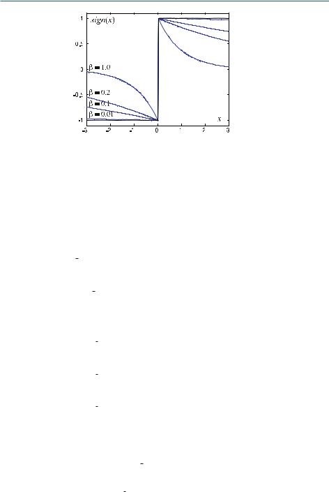
Fig. . . The signum function approximated by a regular sequence of exponential functions. This approximation is necessary to ascertain the convergence of the integrals for explicit application of the Fourier transform
Figure . shows the convergent behavior of the signum function rewritten with the convergence-generating regular sequence. For the decreasing parameter, β, the surrogate function ( . ) tends rapidly toward the original function ( . ).
When calculating the Fourier transform, the transform is first applied to the surrogate function, before applying the limit to the convergence-generating regular sequence.
|
|
|
|
|
|
|
|
|
+ |
|
|
|
|
|
|
|
|
|
|
|
|
|
|
|
|
|
|
|
|
|
|
|
|
|
|
|
|
|
|
|
|
|
|
|
|
||||
|
|
|
|
|
|
α |
|
|
|
∫ sign |
|
|
|
|
|
|
|
|
|
|
|
|
|
|
|
|
|
|
|
|
|
|
|
|
|
|
|
|
|
|
|
|
|
||||||
F |
|
u |
|
|
|
|
|
|
|
x |
|
e−iαux dx |
|
|
|
|
|
|
|
|
|
|
|
|
|
|
|
|
|
|
|||||||||||||||||||
( |
) = π |
|
|
( |
|
|
|
|
|
|
|
|
|
|
|
|
|
|
|
|
|
|
|
||||||||||||||||||||||||||
|
|
|
|
− |
|
. |
|
|
) |
|
|
|
|
|
|
|
|
|
|
|
|
|
|
|
|
|
|
|
|
|
|
|
|
|
. |
( . ) |
|||||||||||||
|
|
|
|
|
|
|
|
|
|
|
|
|
|
|
|
|
|
|
|
|
|
|
|
|
|
|
|
|
|
|
|
|
|
|
|
|
|
|
|
|
|
|
|
|
|||||
|
|
|
|
= |
|
|
|
|
α |
|
|
|
/−− |
|
|
|
|
|
|
|
|
|
|
|
|
|
|
+ |
|
|
|
|
|
|
|
|
|
|
|
C |
|
||||||||
|
|
|
|
βlim |
|
π |
|
|
|
|
- |
|
|
∫ |
|
eβx e−iαux dx |
|
|
∫ e−βx e−iαux dxB . |
|
|||||||||||||||||||||||||||||
|
|
|
|
|
|
|
|
|
|
|
|
|
|
|
0 |
|
|
|
|
|
|
|
|
|
|
|
|
|
|
|
|
|
|
|
|
|
|
|
|
|
|
|
|
|
|
|
|
D |
|
Both of the partial |
integrals in ( . ) can be solved easily. |
|
|
|
|
. |
|
||||||||||||||||||||||||||||||||||||||||||
|
|
|
|
|
|
|
|
. |
|
|
|
|
|
|
|
|
|
|
|
|
|
|
|
|
|
|
|
|
|
|
|
|
|
|
|
|
|
|
|||||||||||
|
|
|
|
|
|
|
|
|
|
|
|
|
|
. |
|
|
|
|
|
|
|
|
|
|
|
|
|
|
|
|
|
|
|
|
|
|
|
|
|
|
|
. |
|
||||||
|
|
|
|
|
|
|
|
|
|
|
|
|
|
|
|
|
|
|
|
|
|
|
|
|
|
|
|
|
|
|
|
|
|
|
|
|
|
|
|
|
|
|
|
|
|
|
|
||
|
( ) = |
|
|
|
|
α |
|
|
|
/−− |
|
|
|
|
|
|
|
|
|
|
|
|
|
+ |
|
|
|
|
|
|
|
|
|
|
|
C |
|
||||||||||||
|
|
|
|
|
|
|
|
|
|
|
|
|
|
|
|
|
|
|
|
|
|
|
|
|
|
|
|
|
|
|
|||||||||||||||||||
F u |
|
βlim |
|
|
π |
|
|
|
- |
|
|
|
∫ |
|
eβx−iαux dx |
|
|
∫ e−(βx+iαux)dxB |
|
||||||||||||||||||||||||||||||
|
|
|
|
|
|
|
|
|
|
α |
|
|
|
. |
|
|
|
|
|
|
|
|
|
|
|
|
|
|
|
|
|
|
|
|
|
|
|
|
|
|
|
|
|
. |
|
||||
|
|
|
|
= |
|
|
|
|
|
|
|
. |
|
|
|
|
|
|
|
|
|
|
|
|
|
|
|
|
|
|
|
+ |
|
|
|
|
|
|
|
|
|
|
. |
|
|||||
|
|
|
|
|
|
|
|
|
|
|
|
|
|
|
|
|
|
|
|
|
|
|
|
|
|
|
|
|
|
|
|
|
|
||||||||||||||||
|
|
|
|
|
βlim |
|
|
π |
|
|
|
- |
|
|
|
∫ |
|
e( |
− |
|
|
) |
x |
dx |
|
∫ |
e−( |
+ |
iαu |
) |
x |
dxB |
( . ) |
||||||||||||||||
|
|
|
|
|
|
|
|
|
|
|
|
|
|
|
0 |
|
|
|
|
|
|
|
|
|
β |
|
|
iαu |
|
|
|
|
|
|
|
β |
|
|
|
D |
|
||||||||
|
|
|
|
|
|
|
|
|
|
|
|
|
|
0 |
|
|
|
|
|
|
|
|
|
|
|
|
|
|
|
|
− |
|
|
|
|
|
|
|
|
|
|
|
|
|
D |
|
|||
|
|
|
|
|
|
|
|
|
|
|
|
|
. |
|
|
|
|
|
|
|
|
|
|
|
|
|
|
|
|
|
|
|
|
|
|
|
|
|
|
|
|
|
. |
|
|||||
|
|
|
|
|
|
|
|
|
|
α |
|
|
|
. |
|
|
|
|
e(β−iαu)x |
|
|
|
|
|
|
|
|
|
e−(β+iαu)x |
|
|
. |
|
||||||||||||||||
|
|
|
|
= |
|
|
|
|
|
|
|
|
/ − |
|
|
|
|
|
|
|
|
|
+ − |
|
|
|
|
|
|
|
|
C |
|
||||||||||||||||
|
|
|
|
|
|
|
|
|
|
|
|
|
|
|
|
|
|
|
|
|
|
|
|
|
|
|
|||||||||||||||||||||||
|
|
|
|
|
βlim |
|
|
π |
|
|
|
. |
|
|
|
|
|
β |
|
|
iαu |
|
|
|
|
|
|
|
|
|
β |
|
iαu |
|
|
|
|
. |
|
||||||||||
|
|
|
|
|
|
|
|
|
|
- |
|
|
|
|
|
|
|
|
|
|
|
|
|
|
|
|
|
|
|
|
|
B . |
|
||||||||||||||||
|
|
|
|
|
|
|
|
|
|
|
|
|
|
|
0 |
|
|
|
|
|
|
|
|
|
|
|
|
|
|
|
|
|
|
|
|
|
|
|
|
|
|
|
|
|
|
|
|
D |
|
The substitution of the interval |
|
|
borders of the integrals and the evaluation of the |
||||||||||||||||||||||||||||||||||||||||||||||
|
|
|
|
− |
|
|
|
|
|
|
|
|
|
|
|
|
|
|
|
|
+ |
|
|
|
|
|
|
|
|
||||||||||||||||||||
limit with respect to β finally results in |
|
|
|
|
|
|
|
|
|
|
|
|
|
|
|
|
|
|
|
|
|
||||||||||||||||||||||||||||
|
|
|
|
|
|
|
|
|
( ) = |
|
|
|
|
|
|
α |
|
|
&− |
|
|
|
|
|
|
+ |
|
|
|
|
|
' |
|
|
|||||||||||||||
|
|
|
|
|
|
|
|
|
|
|
|
|
|
|
|
|
|
|
|
|
|
|
|
|
|||||||||||||||||||||||||
|
|
|
|
|
|
|
|
|
|
|
|
|
|
|
|
|
α |
|
|
|
|
|
|
|
|
|
|
|
|
|
|
− |
|
|
|
|
|
+ |
|
|
|
|
|
|
|
||||
|
|
|
|
|
|
|
F u |
|
|
|
lim |
|
|
|
|
|
|
|
|
|
|
|
|
|
|
|
|
|
|
|
|
|
|
|
|
|
|
|
|
|
|
|
|||||||
|
|
|
|
|
|
|
|
|
|
|
|
|
π |
|
|
|
|
|
|
|
|
β iαu β iαu |
|
|
|
|
|
||||||||||||||||||||||
|
|
|
|
|
|
|
|
|
|
|
|
|
|
|
β |
|
|
|
|
|
|
|
|
|
|
|
|
|
( . ) |
||||||||||||||||||||
|
|
|
|
|
|
|
|
|
|
|
|
|
= |
|
|
|
|
|
|
|
|
|
|
|
|
|
|
|
|
|
|
|
|
|
|
|
|
|
|
|
|
|
|
|
|
||||
|
|
|
|
|
|
|
|
|
|
|
|
|
|
|
|
|
. |
|
|
|
|
|
|
|
|
|
|
|
|
|
|
|
|
|
|
|
|
||||||||||||
|
|
|
|
|
|
|
|
|
|
|
|
|
π |
|
iαu |
|
|
|
|
|
|
|
|
|
|
|
|
|
|
|
|
|
|
|
|
||||||||||||||
|
4 Fundamentals of Signal Processing |
|
|
|
|
||
|
Since α = π is used in the |
later chapters, the result of the transformation is given as |
|||||
|
sign x |
——— |
|
. |
( . ) |
||
|
|
||||||
|
|
|
|
|
iπu |
|
|
|
For more details on regular |
sequences, particularly well-behaved functions and gen- |
|||||
|
( |
) A |
• |
|
|
|
|
eralized functions, the reader is referred to Fichtenholz ( ) or Bracewell ( ).
4.11
Convolution Theorem
An important property of the Fourier transform is given by the convolution theorem. The convolution of the two functions s(x) and h(x),
|
( |
|
) = |
|
( |
|
) > |
|
( |
|
+ |
( |
|
) |
|
( |
|
− |
|
) |
|
|
|
|
|
|
|
|
) =− |
|
|
|
|
|
|
||||||||||
g |
|
x |
|
s |
|
x |
|
h |
|
x |
∫ s |
|
ξ |
|
h |
|
x |
|
ξ |
|
dξ , |
( . ) |
is considered in the spatial domain. To do so, the Fourier transform of ( . ) has to be carried out
( . ) By applying the Fourier transform and permuting the integration order one obtains
+ +
G(u) = ∫ ∫ s(ξ)h(x − ξ)dξ e−i πux dx
− − + +
= ∫ ∫ s(ξ)h(x − ξ)e−i πux dξ dx .
− −
Substituting y = x − ξ and z = ξ into ( . ) gives
+ +
G(u) = ∫ ∫ s(z)h(y)e−i πu(y+z)dz dy
− − + +
= ∫ ∫ s(z)h(y)e−i πu y e−i πuz dz dy .
− −
Both integrals in ( . ) can therefore be separated into two factors, giving
( |
|
+ |
( |
|
) |
+ |
( |
) |
|
|
) =− |
|
− |
|
|||||
G |
u |
∫ h |
|
y |
|
e−i πu y dy ∫ |
s z |
|
e−i πuz dz |
= H(u)S(u) ,
that is
h(x) > s(x) A———• H(u)S(u) ,
and conversely
H(u) > S(u) •———A h(x)s(x) ,
( . )
( . )
( . )
( . )
( . )
The proof of ( . ) can be found, for example, in Klingen ( ). The interested reader is referred to Bracewell ( ) for an extensive discussion of the two-di- mensional convolution theorem.

4.13 Power Theorem |
|
4.12
Rayleigh’s Theorem
The theorem of Rayleigh proves that the integral over the squared modulus of a function is equal to the integral of the squared modulus of its Fourier transform. In the two-dimensional case this can be seen via
+ + |
|
( |
|
) |
|
( |
|
) |
|
+ + |
( |
|
) |
|
( |
|
) |
|
|
|
− − |
|
|
|
|
|
=− − |
|
|
|
|
|
|
||||||||
∫ ∫ |
f |
|
x, y |
|
f |
|
x, y |
|
dx dy |
∫ ∫ f |
|
x, y |
|
f |
|
x, y |
|
e−i π(xu |
+yv |
) dx dy , |
|
|
|
|
|
|
|
|
|
|
|
|
|
|
|
|
|
|
|
|
( . ) |
if u and v are assumed to be zero. The asterisks denote the complex conjugates of the spatial signals and spectra respectively. Using the convolution theorem stated in the section above, the right-hand side of ( . ) is the convolution of the Fourier transforms, i.e., F(u , v ) > F (−u , −v ). Therefore, one obtains
+ + |
( |
|
|
) |
|
( |
|
|
) |
|
|
|
|
|
|
+ + |
( |
|
|
) |
|
|
( |
|
|
− |
|
|
|
− |
|
) |
|
|
||||||
∫ ∫ f |
x, y |
f |
x, y |
dx dy |
|
∫ |
∫ F |
u, v |
F |
u |
u , v |
v |
du dv . |
( . ) |
||||||||||||||||||||||||||
− − |
|
|
|
|
|
|
|
|
|
|
=− − |
|
|
|
|
|
|
|
|
|
|
|
|
|||||||||||||||||
Since u and v are zero, one finally finds that |
|
|
|
|
|
|
|
|
|
|
|
|
|
|
|
|
|
|
||||||||||||||||||||||
+ + |
( |
|
|
) |
|
( |
|
|
|
) |
|
|
|
|
+ + |
( |
|
|
|
) |
|
|
( |
|
|
) |
|
|
|
|
|
|||||||||
∫ |
∫ f |
x, y |
f |
x, y |
dx dy |
|
∫ |
∫ |
F |
u, v |
F |
u, v |
du dv , |
( . ) |
||||||||||||||||||||||||||
− − |
|
|
|
|
|
|
|
|
|
|
=− − |
|
|
|
|
|
|
|
|
|
|
|
|
|
||||||||||||||||
or, more simply, |
|
|
|
|
|
|
|
|
|
|
|
|
|
|
|
|
|
|
|
|
|
|
|
|
|
|
|
|
|
|
|
|
|
|
|
|
||||
|
|
|
|
|
+ + |
|
|
|
|
|
|
|
|
|
|
|
|
+ + |
|
|
|
|
|
|
|
|
|
|
|
|
|
|
|
|||||||
|
|
|
|
|
∫ |
|
∫ |
|
f |
( |
x, y |
) |
dx dy |
|
∫ |
∫ |
|
F |
( |
u, v |
) |
du dv . |
|
( . ) |
||||||||||||||||
|
|
|
|
− − |
|
|
|
|
|
|
|
=− − |
|
|
|
|
|
|
|
|
|
|
|
|
||||||||||||||||
The integrals represent the amount of energy in the system.
4.13
Power Theorem
The power theorem represents a generalized version of Rayleigh’s theorem. By substituting f and f with f and f respectively, one obtains
+ + |
|
( |
|
) |
|
( |
|
) |
|
+ + |
( |
|
) |
|
( |
|
) |
|
|
∫ ∫ |
f |
x, y |
f |
x, y |
dx dy |
∫ ∫ F |
u, v |
F |
u, v |
du dv . |
( . ) |
||||||||
− − |
|
|
|
|
|
=− − |
|
|
|
|
|
Rayleigh’s theorem corresponds to Parseval’s theorem for Fourier series (see Bracewell
).
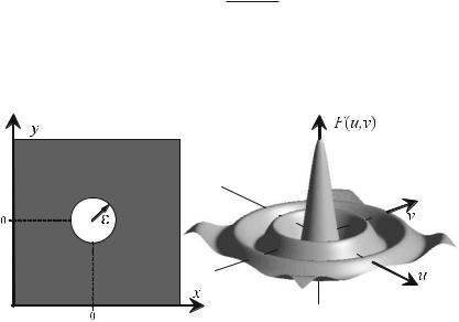
|
4 Fundamentals of Signal Processing |
|
The derivation is the same as for Rayleigh’s theorem. This expression can be inter- |
|
preted as the power or energy of the signal. The left-hand side of ( . ) is evaluated |
|
as the product of a pair of canonically conjugate variables, such as an electric and |
|
magnetic field integrated over space. On the right-hand side, the frequency com- |
|
ponents are multiplied and integrated over the whole spectrum. |
4.14
Filtering in the Frequency Domain
The convolution theorem provides an elegant method of applying filtering in the frequency domain. This will be discussed exemplarily on the basis of a high-pass and a low-pass filtering of an abdominal CT image. First of all, Fig. . provides a description of a circular aperture used for filtering, and the corresponding function in the frequency domain. The result of the high-pass and the low-pass filtering of the image is shown in Fig. . .
In this filtering process, good results still do not come for free. As it has been
shown in |
|
Sect. . , ( . ), the Fourier transform of a rectangular function is |
|
a sinc |
function. This is also reflected by the result of filtering here. Strictly speaking, |
||
|
|
|
|
by applying a circular-rectangular filter, the sine in the result of the sinc function must be replaced by the Bessel function, and so
|
J |
πεq |
|
|
|
F(q) |
|
( q |
) |
, |
( . ) |
where J is the first-order Bessel function, which frequently appears in the solution of problems that have cylindrical symmetry, and q = (u + v ) is the radial frequency variable.
Fig. . . Circular object (left) and the corresponding Fourier transform (right), which is given by the two-dimensional first-order Bessel function of the first kind in ( . )
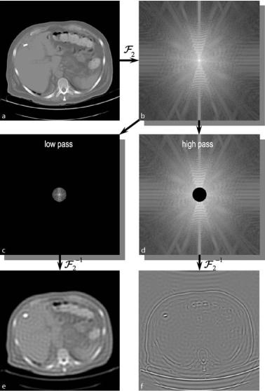
4.14 Filtering in the Frequency Domain |
|
Fig. . . Low-pass (c) and high-pass filtering (d) of an abdominal image (a) using a rectangular filtering function in the frequency domain (b). The figure only provides the magnitude of the complex spectrum in each case. With a circular aperture, only the low (c) or high frequencies (d) respectively remain in the spectrum. Therefore, each complementary spatial frequency is forced to be zero. The inverse transformation back to the spatial domain emphasizes the object’s edges (for the high-pass, f) or results in a slightly blurred image (for the low-pass, e). In addition, one can see in both cases the characteristic waves that seem to emanate from the edges. These waves are, in fact, sidelobes, which are typically produced by sharp-edged filters in the frequency domain

4 Fundamentals of Signal Processing
The Bessel function of the first kind is defined in frequency space by the following integral
Jn (q) = πin |
π |
|
∫ e−iq cos(θ)einθ dθ , |
( . ) |
where n is the order of the Bessel function.
In Fig. . , similar to Fig. . , the Fourier transform of a circular object can be seen. In analogy to the definition of the sinc function – cf. ( . ) – F(q) can alternatively be expressed in terms of the jinc function (Bracewell ), defined as
|
J |
πq |
|
|
|
jinc(q) = |
|
( q |
) |
. |
( . ) |
However, this will not be pursued in detail here. In many books about optics one can find derivations and examples of Bessel functions relating to di raction at a circular aperture.
As a consequence of the filtering, one is able to recognize subsidiary waves of the sinc function, called the sidelobes, in areas of homogeneous gray values. For this reason, window functions are used to counteract these sidelobes. Specific window functions have been examined in detail in the literature (Harris ; Parzen ).
There are numerous proposals for appropriate window functions (such as Hamming, Hanning, Blackman or Kaiser [Azizi ]) that demonstrate less ripple in the result than the rectangular window does. In Sect. . , which is concerned with the technical realization of image reconstruction for CT, the optimal window for filtered backprojection will be considered in detail.
4.15
Hankel Transform
The Hankel transform is a specific type of the two-dimensional Fourier transform with a radially symmetric transform kernel, f (r), where r = (x + y ) . T his type of transform is therefore also referred to as a Fourier–Bessel transform. Starting with the definition given in ( . ) and setting α = π leads to
F(u, v) = |
+ + |
|
∫ ∫ f (r)e− πi(ux+v y)dx dy F f (r) . |
( . ) |
− −
4.15 Hankel Transform |
|
With the problem having radial symmetry, the mathematical description is essentially simplified by introducing polar coordinates. Thus, by substituting
x + iy = r eiθ |
( . ) |
|||||||
and |
|
|
|
|
|
|
|
|
u + iv = q eiϕ , |
( . ) |
|||||||
so that the equations |
|
|
|
|
|
|
|
|
x |
r cos |
θ |
( . ) |
|||||
= |
|
|
|
( ) |
( . ) |
|||
y = r sin (θ ) |
||||||||
r = G |
|
|
|
|
|
|
( . ) |
|
|
x |
|
+ y |
|||||
and |
|
|
|
|
|
|
|
|
u |
q cos |
ϕ |
( . ) |
|||||
= |
|
|
|
( ) |
( . ) |
|||
v = q sin |
(ϕ ) |
|||||||
q = 6 |
|
|
|
|
( . ) |
|||
u |
|
+ v |
||||||
describe the relationship between Cartesian and polar coordinates, ( . ) can be re-written as
|
( |
|
+ + |
|
( |
|
) |
|
|
|
|
|
|
|
|
|
|
|
|
|
|
F |
|
( |
|
) |
|
||||
|
|
) =− − |
|
|
|
|
|
|
|
|
|
|
|
|
|
|
|
|
|
|
|
||||||||||
F |
|
q |
∫ ∫ |
f |
|
r |
|
e− πirq(cos(ϕ)cos(θ)+sin(ϕ)sin(θ))dx dy |
|
|
|
|
f |
|
r |
|
. ( . ) |
||||||||||||||
To carry out the integration, the area element |
dx dy must now be replaced by |
||||||||||||||||||||||||||||||
J dr dθ, where J is called the Jacobian, i.e., |
|
|
|
|
|
|
|
|
|
|
|
|
|
|
|
|
|
||||||||||||||
|
|
|
|
|
|
|
|
|
|
|
|
∂x |
|
∂y |
|
|
|
|
|
|
|
|
|
|
|
|
|
|
|
|
|
|
|
|
|
|
|
|
|
|
( ) |
= |
∂θ ∂θ |
= 9 |
− |
|
|
|
( ) |
|
( ) 9 |
|
|
||||||||||
|
|
|
J |
|
det |
|
|
∂ x, y |
|
∂r |
|
∂r |
|
|
cos |
θ |
|
sin |
|
θ |
|
|
|
|
|
|
|||||
|
|
|
|
|
|
|
|
|
|
∂(r, θ ) |
|
∂x |
|
∂y |
|
|
|
r |
sin |
|
θ r cos |
θ |
|
|
|
( . ) |
|||||
|
|
|
|
|
|
|
|
|
|
= Hr |
|
|
|
|
|
( |
|
) |
|
( |
|
) |
|
|
|
||||||
|
|
|
|
|
|
|
|
|
|
|
cos (θH) + sin (θ) = r . |
|
|
|
|
|
|
|
|
||||||||||||
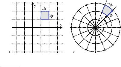
|
4 Fundamentals of Signal Processing |
In Fig. . the calculation of the infinitesimal area element can be seen graphically.
This leads to
+ π |
f (r)e− πirq(cos(ϕ)cos(θ)+sin(ϕ)sin(θ))r dθ dr F f (r) . |
|
||
F(q) = ∫ |
∫ |
( . ) |
||
Using the addition law of the cosine |
|
|||
it follows that |
|
cos(α $ β) = cos(α)cos(β) % sin(α)sin(β) , |
( . ) |
|
|
|
+ π |
|
|
|
|
F(q) = ∫ |
∫ f (r)e− πirq(cos(θ−ϕ))r dθ dr . |
( . ) |
The constant phase shift about the angle ϕ in the argument of the cosine, can be removed by shifting the integration limits, giving
F(q) = |
+ π−ϕ |
|
|
∫ |
∫ f (r)e− πirq(cos(θ))r dθ dr . |
( . ) |
|
|
|
−ϕ |
|
Since the integrand of ( . ) is radially symmetric, the phase shift can be neglected so that, after resorting the integrands, one obtains
|
( |
|
) = |
+ |
( |
) |
π |
e− πirq(cos(θ))dθ |
" |
|
|
|
|
|
|
|
|||||||
F |
|
q |
|
∫ f |
r |
|
∫ |
! r dr . |
( . ) |
||
|
|
|
|
|
|
|
|
|
|
# |
|
|
|
|
|
|
|
|
|
|
|
|
|
|
|
|
|
|
|
|
|
|
|
|
|
|
|
|
|
|
|
|
|
|
|
|
|
Fig. . . The formation of an infinitesimal area element after transformation from a Cartesian to b polar coordinates
It simply represents an initial angle in an integration over one full rotation.

4.15 Hankel Transform |
|
The term in the bracket in ( . ) is just the th order Bessel function of the first kind – defined in general in ( . ) –, i.e., in the frequency space
J (q) = |
|
|
π |
|
|
∫ e−iq cos(θ)dθ |
( . ) |
||||
π |
|||||
thus, one may write |
|
|
|
|
|
|
+ |
f (r)J ( πqr)r dr . |
|
||
F(q) = π ∫ |
( . ) |
||||
( . ) is known as the Hankel transform. It is a one-dimensional transform since f and F are functions of one variable. However, as functions of one variable, they may also represent two-dimensional functions.
To complete the description of the th order Hankel transform, the inverse transform given as
+ |
|
f (r) = π ∫ F(q)J ( πqr)q dq |
( . ) |
is needed. The pair of Hankel transform equations are conventionally denoted by
and |
F(q) = H f (r) |
( . ) |
|
f (r) = H F(q) . |
( . ) |
In fact, Fig. . from the section above is an example of the Hankel transform, i.e., the Hankel transform of a disk
|
f (r) = rect |
r |
|
|
( . ) |
|||
is given by |
ε |
|||||||
|
|
εJ |
πεq |
|
|
|
||
|
F(q) = |
|
( q |
|
|
) |
. |
( . ) |
The rectangular function, rect(r), has the Hankel transform jinc(q), shown in integral formulation
+ |
|
jinc(q) = π ∫ rect(r)J ( πqr)r dr |
( . ) |
and |
|
+ |
|
rect(r) = π ∫ jinc(q)J ( πqr)q dq |
( . ) |
respectively.
4 Fundamentals of Signal Processing
4.16
Abel Transform
Computed tomography of rotationally symmetric objects results in a mathematically interesting transform, which is closely connected to both the Hankel transform and the Fourier transform. In the case of the projections of a radially symmetric
object space object space
f (x,y) f(x,y)
object space object space
f (r) f(r)
projection projection
p (x) p(x)
a
2–1
2
0
1
1–1
r
Fourier space Fourier space
F (u, v) F(u,v)
Fourier space Fourier space
P(q) P(q)
0
1
x |
q |
b
Fig. . . a Relationship between the Fourier transform, the Hankel transform, and the Abel transform. The Hankel transform can be replaced by the Abel transform and a subsequent one-dimensional Fourier transform. b Example of the Fourier–Abel–Hankel cycle using jinc(r)

4.17 Hilbert Transform |
|
object, ( . ) can be simplified, since the projection onto the x-axis is given by
|
|
|
|
( |
|
|
+ |
|
|
( |
) |
|
|
||
|
|
|
|
|
) =− |
|
|
|
|
||||||
|
|
p |
|
x |
|
∫ |
|
f |
r |
|
dy , |
||||
where the radius r is given by ( . ). Substituting |
|
||||||||||||||
|
|
|
|
|
y = |
6 |
|
|
, |
|
|||||
gives |
|
|
|
|
r − x |
|
|||||||||
|
( |
|
) = |
|
+ |
6 |
|
|
|
|
|
||||
p |
x |
|
x∫ |
|
|
|
dr . |
||||||||
|
− |
|
|||||||||||||
|
|
|
|
|
fr(r)rx |
||||||||||
( . )
( . )
( . )
From ( . ) it is clear that the minimum radius is x. T he factor in ( . ) is due to contributions from values above and below the x-axis.
( . ) is referred to as the Abel transform of the object f (r). The Abel transform is conventionally denoted by
|
|
|
|
|
p |
x |
|
|
f |
r . |
|
|
|
|
|
( . ) |
||
|
|
|
|
|
|
function, |
f x, y |
|
|
|
f |
r , the relationship in |
||||||
For a radially symmetric object ( ) = A |
|
( ) |
|
) |
|
= |
|
( ) |
|
|||||||||
Fig. . holds. |
|
|
|
|
|
|
|
|
|
( |
|
|
|
|
|
|||
It follows that |
|
|
|
|
|
|
|
|
|
|
|
|
|
|
|
|
|
|
|
|
|
|
f r |
|
|
|
|
f |
|
r |
|
|
|
|
|
( . ) |
|
also holds. ( . ) is called the |
Fourier–Abel–Hankel cycle. Since the Fourier–Abel– |
|||||||||||||||||
|
( ) = H |
|
F A ( ) |
|
|
|
|
|
||||||||||
Hankel operation is cyclic, it holds that |
|
|
|
|
|
|
|
|
|
|
|
|
||||||
I |
|
|
|
|
|
|
|
|
|
|
|
|
|
|
|
|
|
( . ) |
operator. |
|
|
|
|
|
|
|
|
|
|
|
|
|
|||||
where is the identity |
H |
|
F A = AH F = F AH = I |
|
|
|||||||||||||
4.17
Hilbert Transform
The Hilbert transform of a function, |
|
|
is defined |
by |
|
|
|
|
|
|
||||||||||||
|
|
|
|
|
|
|
|
|
f (x)+, |
|
x |
|
|
|
|
|
|
|
|
|||
|
|
|
|
|
( |
|
) = |
|
|
f |
|
|
|
|
|
|
|
|
||||
|
|
H |
f |
x |
π |
− |
( |
x) dx |
. |
|
|
( . ) |
||||||||||
|
|
|
|
|
|
|
∫ x |
|
|
|||||||||||||
|
|
|
|
|
|
|
|
|
|
|
|
− |
|
|
the sense of |
|||||||
|
Due to the divergence at x = x |
|
|
|
|
|
|
|
|
|
||||||||||||
|
|
|
the integral ( . ) needs to be interpreted in |
x −ε |
|
|
|
|||||||||||||||
|
|
|
|
|
|
|
|
|
|
|
|
|
|
|
|
ε |
|
∫ |
+x |
|
∫+ε |
|
|
Cauchy’s fundamental theorem (Bronstein and Semendjajew ), i.e., lim |
− |
|
|
||||||||||||||||||
|
|
|
|
|
|
. |
||||||||||||||||
|
|
|
|
|
|
|
|
|
|
|
|
|
|
|
|
|
|
|
|
|
|
|
|
|
|
|
|
|
|
|
|
|
|
|
|
|
|
|
|
|
|
|
|
|
|
|
4 Fundamentals of Signal Processing |
|
|
|
|
|
|
|
|
|
|
|
|
|
|
|
|
|
|
|
|
|
||||||||||||||||||
|
It should be noted that the definition in ( . ) describes a convolution of the func- |
|||||||||||||||||||||||||||||||||||||||
|
tion f |
|
x |
|
|
with the function |
|
|
πx |
− |
|
|
|
|
|
|
|
|
|
|
|
|
|
|
|
|
|
|
|
|
|
|||||||||
|
|
|
|
( |
|
) |
|
|
|
|
|
(H )f |
x, i.e., |
|
|
|
|
|
f |
x . |
|
|
|
|
|
( . ) |
||||||||||||||
|
|
|
|
|
|
|
|
|
|
|
πx |
|
|
|
|
|
|
|||||||||||||||||||||||
|
This convolution can be applied in the frequency domain. Therefore, one needs to |
|||||||||||||||||||||||||||||||||||||||
|
|
|
|
|
|
|
|
|
|
|
|
|
|
|
|
|
( |
) = |
|
|
|
|
|
> |
|
( |
) |
|
|
|
|
|
|
|
|
|||||
|
recall the derivation of the transform ( . ) and apply it to the signum function in |
|||||||||||||||||||||||||||||||||||||||
|
the frequency domain. This gives |
|
|
|
|
|
|
|
|
- |
|
|
|
|
|
|
|
|
|
|
|
|
||||||||||||||||||
|
|
|
|
|
|
|
|
|
|
|
|
|
|
|
|
|
|
|
|
|
|
|
|
|
|
|
i |
for positive u |
|
|
|
|||||||||
|
|
|
|
|
|
|
|
|
|
——— |
|
|
|
i sign u |
|
|
|
|
|
for u |
|
|
|
|
|
( . ) |
||||||||||||||
|
|
|
|
|
|
|
|
|
πx |
|
|
|
|
|
|
|
|
|
|
|
||||||||||||||||||||
|
|
|
|
|
|
|
|
|
|
|
|
• − |
|
|
|
|
|
|
|
|
|
. |
−i |
for negative u |
|
|
|
|||||||||||||
|
|
|
|
|
|
|
|
|
|
A |
|
|
|
|
|
|
( ) = / |
|
|
|
|
|
= |
|
|
|
|
|
|
|||||||||||
|
In this way, the Hilbert transform has the properties of not altering the amplitude, |
|||||||||||||||||||||||||||||||||||||||
|
|
|
|
|
|
|
|
|
|
|
|
|
|
|
|
|
|
|
|
|
|
|
|
|
|
|
. |
+ |
|
|
|
|
|
|
|
|
|
|
|
|
|
|
|
|
|
|
|
|
|
|
|
|
|
|
|
|
|
|
|
|
|
|
|
|
|
|
|
0 |
|
|
|
|
|
|
|
|
|
|
|
|
|
|
but of shifting the phase by |
|
|
π or |
|
|
π respectively (according to the sign of u). |
|||||||||||||||||||||||||||||||||
|
Instead of carrying out the integral in ( . ), the Hilbert transform is obtained via |
|||||||||||||||||||||||||||||||||||||||
|
|
|
|
|
|
|
|
|
|
|
|
|
+ |
|
|
|
|
|
− |
|
|
|
|
|
|
|
|
|
|
|
|
|
|
|
|
|
||||
|
the convolution theorem. Let |
|
|
F(u) = F f (x) , |
|
|
|
|
|
|
|
|
|
|||||||||||||||||||||||||||
|
then |
|
|
|
|
|
|
|
|
|
|
|
|
|
|
|
|
|
|
|
|
|
( . ) |
|||||||||||||||||
|
|
|
|
|
|
f |
x |
|
H f x |
|
|
|
|
|
H |
|
|
|
|
f |
|
x |
|
|
|
H |
F u |
|
i sign |
u |
F |
u . |
||||||||
|
|
πx |
|
|
|
|
|
|
|
|
|
|
|
|
|
|
|
|
|
|||||||||||||||||||||
|
|
|
|
|
|
|
|
|
|
|
|
|
|
|
|
|
|
|
|
|
|
|
|
|
|
|
|
|
|
|
|
|
|
|
|
. ) |
||||
|
FM |
|
|
> |
|
( )O=F |
|
( ) = |
|
|
F ( ) = |
|
|
|
( |
) =− ċ |
( )ċ |
|||||||||||||||||||||||
|
|
|
|
|
|
|
|
|
(( |
) |
||||||||||||||||||||||||||||||
|
The Hilbert transform is thus obtained by |
|
|
|
|
|
|
|
|
|
|
|
|
|
|
|
|
|||||||||||||||||||||||
|
|
|
|
|
|
|
|
|
|
H f |
x |
|
|
|
|
|
− |
|
i |
|
sign |
|
u |
|
F |
u . |
|
( . ) |
||||||||||||
|
By applying the Hilbert transform twice in succession, the phases become inverted, |
|||||||||||||||||||||||||||||||||||||||
|
|
|
|
|
|
|
|
|
|
|
|
( ) = F |
|
|
|
− ċ |
|
|
|
( ) ċ ( ) |
|
|
|
|
||||||||||||||||
|
with the final result being the negative of the original function, thus |
|
|
|
||||||||||||||||||||||||||||||||||||
|
|
|
|
|
|
|
|
|
|
|
|
|
H |
H f |
(x) = −f (x) . |
|
|
|
|
|
( . ) |
|||||||||||||||||||
This can be derived in the frequency domain as well. |
|
|
|
|
|
|
|
|
|
|
|
|
||||||||||||||||||||||
F |
|
|
f |
( |
x |
) = |
|
|
|
i |
|
F |
( |
u |
) |
|
|
|
|
|
|
|
|
|
|
|
|
|||||||
H |
H |
|
|
|
= |
H |
|
H |
|
|
|
|
|
) ċ |
|
|
( |
|
|
) |
|
|
|
|
||||||||||
|
|
|
|
|
|
|
|
i |
− ċ |
sign |
( |
u |
|
F |
u |
|
|
|
|
|||||||||||||||
|
|
|
|
|
|
|
|
H |
|
|
|
|
|
|
|
i |
( |
) |
|
|
|
|
||||||||||||
|
|
|
|
|
|
|
= −i |
ċ sign(u) ċ |
|
F |
u |
|
|
|
|
|||||||||||||||||||
|
|
|
|
|
|
|
|
|
|
|
sign |
|
u |
|
|
|
H |
|
|
|
|
) ċ |
|
( |
|
) |
||||||||
|
|
|
|
|
|
|
= −Fċ u .( ) ċ − ċ |
sign |
( |
u |
F |
u |
||||||||||||||||||||||
|
|
|
|
|
|
|
|
|
|
|
|
|
|
|
|
|
|
|
|
|
|
|
|
|
|
|
|
|||||||
|
|
|
|
|
|
|
obtained by |
|
|
|
|
|
|
|
|
|
|
|
|
|
|
|
|
|
|
|||||||||
Therefore, the inverse transform is = − |
( |
) |
|
|
|
|
|
|
|
|
|
|
|
|
|
|
|
|
|
|
|
|
|
|||||||||||
|
|
|
|
f (x) = − |
|
|
> H f (x) , |
|
|
|
|
|
|
|
|
|
|
|||||||||||||||||
or alternatively |
|
|
|
πx |
|
|
|
|
|
|
|
|
|
|
||||||||||||||||||||
|
|
|
|
( ) = − |
− |
|
|
|
|
−( |
) |
|
|
|
|
|
|
|
|
|
|
|
|
|
||||||||||
|
|
|
|
|
|
|
|
+H |
|
|
f |
x |
|
|
|
|
|
|
|
|
|
|
|
|
|
|
|
|||||||
|
|
f |
x |
|
π |
|
∫ |
|
|
|
x |
|
|
x |
|
|
|
dx . |
|
|
|
|
|
|
|
|
|
|||||||
|
|
|
|
|
|
|
|
|
|
|
|
|
|
|
|
|
|
|
|
|
|
|
|
|
|
|
|
|
||||||
( . )
( . )
( . )
As a consequence, four successive Hilbert transforms result in the identity operation, i.e.,
HHHH = I . ( . )
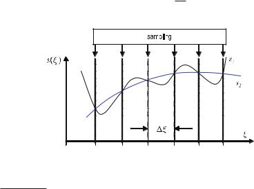
4.18 Sampling Theorem and Nyquist Criterion |
|
4.18
Sampling Theorem and Nyquist Criterion
Due to sampling, a continuous signal is transformed into a digital one. The resulting, spatially discrete signal only coincides with the continuous signal, for instance, the continuously distributed attenuation coe cients at the sampled points. The signal values situated between the sample points are not captured. In this section, it will be briefly considered how accurately the continuous spatial signal, s(ξ), needs to be sampled, in order to measure a discrete signal, si , that su ciently represents the original one.
Figure . shows that it is always possible to construct di erent continuous functions passing all sample points as long as the sampling interval is larger than zero. For this reason, quite di erently shaped functions might look identical after sampling, i.e., the sampling is not unique (Stearns and Hush ).
The question of which changes in information content the continuous signal experiences due to sampling can be answered by means of the Nyquist–Shannon sampling theorem.
According to the Nyquist–Shannon sampling theorem, the sampled signal bears the same amount of information as the continuous signal if the sampling frequency is larger than twice the highest frequency (or alternatively the bandwidth of bandlimited signals) contained in the spectrum of the continuous signal. In other words, a signal, s(ξ), must be sampled at least twice during the cycle with its highest frequency.
In this way, if the signal s(ξ) satisfies
S(u) = for u : |
uN |
, |
( . ) |
|
Fig. . . Di erent functions with identical sampling points. Both functions share the same sampled values, although the shapes of the two functions are quite di erent
However, a digital signal is not achieved alone from sampling, since it requires quantization as well.

|
4 Fundamentals of Signal Processing |
then the sampling rate must be larger than uN, which is called the Nyquist frequency. This criterion protects against errors due to band overlap, the “aliasing”, where a high-frequency signal digitized at too low a sampling rate will be indistinguishable from a low frequency signal. In two dimensions this phenomenon is referred to as the Moiré e ect. With a predetermined sampling period, the signal needs to be filtered by a corresponding low-pass filter (Azizi ). For practical applications, one has to keep in mind that the sampling theorem is a theoretical statement that does not take into account the violation of certain assumptions, including quantization errors or spatial irregularities of the arrangement of the sampling points (jitter) (Kiencke ).
The sampling theorem can be justified in the frequency domain by considering a signal that has been sampled using the comb function,
|
( |
) = |
+ |
( |
|
) ( |
|
− |
|
) = |
( |
) |
+ |
( |
|
− |
|
|
) = |
( |
) |
( |
) |
|
sa |
|
n |
ξ |
n ξ |
|
ξ |
n |
ξ |
, ( . ) |
|||||||||||||||
ξ |
|
n =− |
s |
ξ δ |
|
|
s ξ |
|
n =− |
δ |
|
|
s ξ |
|
Ш ξ |
|
||||||||
|
|
|
|
|
|
|
|
|
|
|
|
|
|
|
|
|
|
|
|
|
|
|
in the spatial domain. In ( . ), the spatial coordinate, ξ, is continuous and the discrete sequence values, s(n ξ), are the strengths of the impulses located at each sample point.
Here, one initially calculates the Fourier transform of the comb function (Lüke; Klingen ), which gives another comb function. This result can be understood by means of the relations introduced earlier. First, according to ( . ), the Fourier transform of the comb function gives
|
F |
|
( − |
|
|
|
) = |
|
− πiun ξ |
|
|
|||||||||
|
|
|
+ |
δ |
|
ξ |
|
|
n |
|
ξ |
|
|
+ |
|
. |
( . ) |
|||
|
|
|
|
|
|
|
|
|
|
|
|
|
e |
|||||||
|
|
n =− |
|
|
|
|
|
|
|
|
n =− |
|
|
|
||||||
Writing the right hand side of ( . ) as a limit |
|
|
|
|
|
|||||||||||||||
|
|
+ |
|
|
− πiun ξ |
= |
|
|
|
N |
|
− πiun ξ |
|
|
||||||
|
|
|
|
e |
|
|
|
|
|
|
|
lim |
|
e |
|
|
( . ) |
|||
|
= |
n =− |
|
|
|
|
) |
|
|
N n =−N |
|
|
|
|||||||
and substituting ψ |
exp |
(− |
πiu |
|
ξ |
such that, |
|
|
|
|
|
|||||||||
|
|
|
|
|
|
|
|
|
|
|||||||||||
|
|
|
+ |
|
|
|
|
|
|
|
|
= |
|
|
N |
|
|
|
||
|
|
|
|
|
e− πiun |
ξ |
lim |
|
ψn , |
|
( . ) |
|||||||||
|
|
|
n =− |
|
|
|
|
|
|
|
|
N n =−N |
|
|
||||||
the right-hand side of ( . ) can be represented as the limit of a geometric series (Papula ), namely
N
lim ψn =
N n =−N
=
=
lim
N
lim
N
lim
N
ψ−N |
− ψ |
N+ |
|
|
|
|
|
|
|
|
|
|
|||
|
ψ |
|
|
|
|
|
|
|
|
|
|
||||
|
πiu ξN− |
e− πiu ξ( N+ ) |
|
|
|
|
|
|
|
||||||
e |
|
|
|
|
− |
e− πiu |
ξ |
+ |
− |
|
− |
|
( . ) |
||
|
|
|
e−πiu− |
− |
|
|
|
|
|
||||||
e πiu ξN |
|
|
|
|
|
|
|
|
|
|
. |
||||
|
|
|
|
|
|
e πiu ξ e πiu ξ |
|
e−πiu ξ |
|
|
|
||||
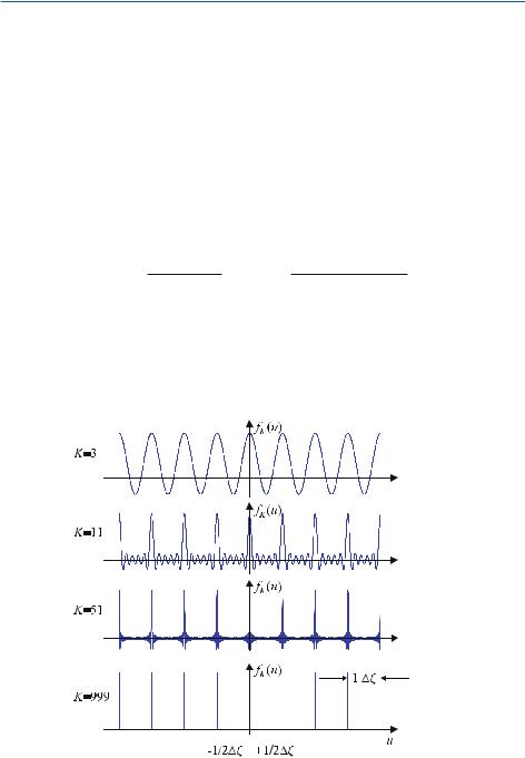
4.18 Sampling Theorem and Nyquist Criterion
With K = N + , |
one obtains the expression |
|
|
|
|
|
|
|
|
|
|
|
|
|
|
|
|
|
||||||||||||||||||||||||||
|
|
|
+ |
|
|
( |
|
− |
|
|
|
) = |
|
|
|
|
|
e+Kπiu |
ξ |
|
e−Kπiu |
|
ξ |
|
|
|
||||||||||||||||||
and further |
|
F |
|
|
|
δ |
ξ |
|
n |
ξ |
|
lim |
|
|
|
|
− |
|
|
|
|
|
|
|
|
( . ) |
||||||||||||||||||
|
|
|
|
|
|
n =− |
|
|
|
|
|
|
|
|
|
|
|
|
K |
|
|
e+πiu ξ − e−πiu ξ |
|
|
|
|||||||||||||||||||
|
|
|
|
|
F |
+ |
|
|
|
( |
|
|
− |
|
|
|
) = |
|
|
|
|
|
sin |
|
Kπu |
ξ |
|
|
|
|
|
|
|
|||||||||||
|
|
|
|
|
|
|
|
δ |
ξ |
n |
|
ξ |
lim |
|
|
|
|
|
|
|
|
. |
|
|
( . ) |
|||||||||||||||||||
|
|
|
|
|
|
|
|
|
|
|
|
|
|
|
|
|
|
|
|
|
|
|
|
sin |
πu |
|
|
ξ |
) |
|
|
|
||||||||||||
|
|
|
|
|
|
|
|
|
n =− |
|
|
|
|
|
|
|
|
|
|
|
|
|
|
|
|
|
|
|
|
|
|
|
|
|||||||||||
|
|
|
|
|
|
|
|
|
|
|
|
|
|
|
|
|
|
|
|
|
|
|
|
|
|
K |
|
|
|
|
|
|
|
|
|
|
|
|
|
|
|
|
|
|
|
|
|
|
|
|
|
|
|
|
|
|
|
|
|
|
|
|
|
|
|
|
|
|
|
|
|
|
|
|
|
|
|
|
|
|
|
) does not change if |
|||||||
Since K is an integer, the result on the right-hand side(of ( . ) |
|
|
|
|
|
|
||||||||||||||||||||||||||||||||||||||
the quantity |
|
u ξ |
|
|
is replaced by |
|
u |
|
ξ |
|
n , where n is also an integer, as sine is |
|||||||||||||||||||||||||||||||||
a periodic |
function and the zeros of the numerator and the denominator still appear |
|||||||||||||||||||||||||||||||||||||||||||
|
|
( |
|
|
) |
( |
|
|
|
) |
|
|
|
|
|
|
( |
|
|
|
|
− |
|
) |
|
|
|
|
|
|
|
|
|
|
|
|
|
|
|
|
|
|||
at integer numbers, |
u ξ |
. T hus, it holds that |
|
|
|
|
|
|
|
|
|
|
|
|
|
|
|
|
||||||||||||||||||||||||||
|
|
|
|
|
|
|
|
|
|
|
|
|
|
|
|
|
|
|||||||||||||||||||||||||||
|
|
|
( ) = |
|
|
|
|
sin |
( |
|
|
|
|
|
) |
= |
|
|
|
sin |
( |
( |
|
|
− )) |
|
|
|||||||||||||||||
|
|
|
|
|
|
|
|
( |
|
|
|
|
) |
|
|
|
|
|
|
( ( |
|
|
|
− )) |
|
|||||||||||||||||||
lim fK |
|
u |
|
|
lim |
|
|
sin |
|
πu |
|
ξ |
|
|
|
|
|
lim |
|
|
|
sin |
π |
|
u |
ξ |
|
n |
|
|
. ( . ) |
|||||||||||||
K |
|
|
|
|
|
K |
|
|
|
|
|
|
|
|
|
|
|
|
|
|
|
|
|
|
K |
|
|
|
|
|
|
|
|
|
|
|
|
|
|
|
|
|
|
|
( . ) also implies that, due to translation invariance, there is a fundamental interval, (− ξ, + ξ), which repeats itself periodically. This means that the function ( . ) is indeed identical within the intervals ( n − ξ, n + ξ) for all integer numbers, n ; Z. Figure . shows the shape of fK (u) in ( . ) for an increasing parameter K = , , , .
Fig. . . The function fK(u) tends toward the comb function for increasing parameter K. In this way, it is shown that the Fourier transformation of the comb function is once again a comb function
|
4 |
Fundamentals of Signal Processing |
|
|
|
|
|
|
|
|
|
|
|
|
|
|
|
|
|
|
|
|
|
|
|
|
|
|
|
|
|
|
|
|
|
|
||||||||||||||||||
|
|
For each n Z, in the neighborhood of |
|
u |
|
|
ξ |
|
n |
|
|
|
|
, one can approximate the |
||||||||||||||||||||||||||||||||||||||||
|
|
|
|
|
|
|
|
|
|
|
|
|
|
|
|
|
|
|
|
|
|
|
|
|
|
|
|
|
|
|
|
|
|
Taylor expansion, i.e., |
|
|
||||||||||||||||||
|
denominator in;( . ) with the linear term(of its− |
|
|
) = |
|
|
|
|
|
|
|
|
|
|
|
|
|
|
||||||||||||||||||||||||||||||||||||
|
|
|
|
|
|
|
|
|
|
|
sin |
|
π u |
ξ |
|
|
n |
|
|
|
|
π u |
|
ξ |
|
|
|
n |
|
, |
|
|
|
|
|
|
|
|
|
|
|
( . ) |
||||||||||||
|
so that, by means of |
definitions ( . ) and ( . ) of the δ-distribution, |
|
|
||||||||||||||||||||||||||||||||||||||||||||||||||
|
|
|
|
|
( |
|
( |
|
|
|
− |
|
|
|
)) |
|
|
( |
|
|
|
|
− |
|
|
) |
|
|
|
|
|
|
|
|
|
|
|
|
|
|||||||||||||||
|
|
|
( |
|
|
|
|
|
|
|
|
|
|
= |
|
|
|
|
|
ε |
|
|
|
|
|
|
|
|
|
|
= |
|
|
|
|
|
|
sin |
|
πεu |
|
|
|
|
||||||||||
|
|
δ |
u |
) =− |
|
e−i πux dx |
|
lim |
− |
|
|
|
e−i πux dx |
|
|
lim |
|
|
|
|
|
( . ) |
||||||||||||||||||||||||||||||||
|
|
|
|
∫ |
|
|
|
|
|
|
|
|
|
|
|
|
|
|
|
|
|
|
( |
|
|
|
) |
|
||||||||||||||||||||||||||
|
|
|
|
|
|
|
|
|
|
|
|
|
|
|
ε |
ε |
|
|
|
|
|
|
|
|
|
|
|
|
|
|
ε |
|
|
|
|
|
|
|
|
|
|
|||||||||||||
|
|
|
|
|
|
|
|
|
|
|
|
|
|
|
|
|
|
∫ |
|
|
|
|
|
|
|
|
|
|
|
|
|
|
|
|
|
|
|
|
|
πu |
|
|
|
|
|
|||||||||
|
it follows that |
|
|
K |
|
|
|
|
(π u( ξ n− |
|
|
)) = ( |
|
|
|
|
|
− ) |
|
|
|
|
|
|
|
|||||||||||||||||||||||||||||
|
|
|
|
|
|
|
|
sin |
n |
|
|
|
|
|
|
|
|
|
|
|
|
|||||||||||||||||||||||||||||||||
|
|
|
|
|
|
|
|
lim |
|
|
Kπ |
|
u |
|
|
ξ |
|
|
|
|
|
|
|
|
δ u |
|
ξ |
|
|
|
n , |
|
|
|
|
( . ) |
||||||||||||||||||
|
|
( − |
|
|
|
|
|
|
|
|
|
|
|
|
|
|
|
|
|
|
|
; |
|
|
|
|
|
|
|
|
|
|
|
|
|
|
||||||||||||||||||
|
|
|
|
+ ] |
|
|
|
all n |
Z. Since ( . ), as already discussed |
|||||||||||||||||||||||||||||||||||||||||||||
|
for |
n |
|
ξ, |
|
n |
|
|
|
|
|
ξ( and− ) |
|
|
|
|
|
|
|
|
|
|
|
|
|
|
|
|
|
|
|
|
|
|
|
|
|
|
|
|
||||||||||||||
|
above, is periodic – repeating the fundamental interval |
|
|
|
|
|
|
ξ, ξ |
|
– and |
||||||||||||||||||||||||||||||||||||||||||||
|
e ective for arbitrary integer, n, (cf. Fig. . ), the |
|
expression on the right-hand |
|||||||||||||||||||||||||||||||||||||||||||||||||||
|
|
|
|
|
|
|
(− |
|
|
|
+ |
] |
|
|||||||||||||||||||||||||||||||||||||||||
|
side must be interpreted as a sequence of δ-impulses, allowing us to write |
|
|
|||||||||||||||||||||||||||||||||||||||||||||||||||
|
|
|
|
|
|
|
F |
+ |
|
|
|
( |
|
|
− |
|
|
|
|
|
) = |
|
|
|
+ |
|
|
|
|
( |
|
|
|
|
|
− |
|
) |
|
|
|
|
|
|
|
|||||||||
|
|
|
|
|
|
|
|
|
δ |
ξ |
n |
|
ξ |
|
|
|
|
|
|
δ |
u |
|
ξ |
|
n |
|
. |
|
|
|
|
( . ) |
||||||||||||||||||||||
|
|
|
|
|
|
|
|
|
|
n =− |
|
|
|
|
|
|
|
|
|
|
|
|
|
|
|
|
n =− |
|
|
|
|
|
|
|
|
|
|
|
|
|
|
|
|
|
|
|
||||||||
|
This, along with the scaling property ( . ), gives |
|
|
|
|
|
|
|
|
|
|
|
|
|
|
|
|
|
|
|
|
|
||||||||||||||||||||||||||||||||
|
|
|
|
|
|
F |
+ |
|
|
( |
|
− |
|
|
|
) = |
|
|
|
|
+ |
|
|
|
− |
n |
|
|
|
|
|
|
|
|||||||||||||||||||||
|
|
|
|
|
|
|
|
|
|
|
|
|
|
|
|
|
|
|
|
|
|
|
. |
|
|
|
( . ) |
|||||||||||||||||||||||||||
|
|
|
|
|
|
|
|
|
|
|
δ |
|
ξ |
|
|
|
n |
|
ξ |
|
|
|
|
|
|
|
|
|
|
|
|
|
|
|
|
|
δ |
u |
|
|
|
|
|
|
|
|
|
|
||||||
|
|
|
|
|
|
|
|
|
n =− |
|
|
|
|
|
|
|
|
|
|
|
|
|
|
|
|
|
ξ |
|
n =− |
|
|
|
|
|
|
|
|
ξ |
|
|
|
|
|
|
||||||||||
Taking advantage of the convolution theorem ( . ) and by means of ( . ) for sampling ( . )
|
( |
|
) = |
|
( |
|
) |
+ |
|
( |
|
− |
|
sa |
ξ |
s |
ξ |
|
δ |
ξ |
n |
||||||
|
|
|
|
|
|
|
|
n =− |
|
|
|
|
|
in the frequency domain, one obtains the expression
|
( |
|
) = |
|
( |
|
) > |
|
+ |
|
|
|
− |
Sa |
u |
S |
u |
|
|
δ |
u |
||||||
|
|||||||||||||
|
|
|
|
ξ n =− |
|
|
|||||||
|
|
|
|
|
|
|
|
|
|
|
|
||
The convolution can be written explicitly as
ξ) |
|
( . ) |
|
|
n |
. |
( . ) |
|
ξ |
||
|
|
|
|
|
|
|
|
|
+ |
|
|
|
|
n |
− |
|
|
|
|
|
( |
|
) =− |
|
( |
|
) |
|
|
|
− |
|
|
|
|||||
|
|
|
|
|
|
|
|
|
|
|
|
||||||||
Sa |
|
u |
∫ |
S |
|
v |
|
ξ |
n =− |
δ |
|
u |
|
ξ |
|
v |
|
dv , |
( . ) |
|
|
|
|
|
|
|
|
|
|
|
|
|
|
|
|
|
|
|
so that, by permuting the summation and the integration in ( . ),
|
( |
|
) = |
|
+ |
|
|
( |
|
) |
|
|
|
− |
n |
− |
|
|
|
|
|
|
|
|
− |
|
|
|
|
|
|
|
|
||||||||
Sa |
|
u |
|
ξ |
|
∫ |
S |
|
v |
|
δ |
|
u |
|
ξ |
|
v |
|
dv |
( . ) |
|
|
|
|
|
n =− |
|
|
|
|
|
|
|
|
|
|
|
|
|
|
|
can be obtained.
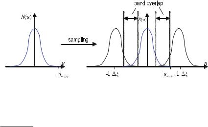
4.18 Sampling Theorem and Nyquist Criterion |
|
Once again, the final result is obtained by means of the sift property of the δ- distribution, thus
|
( |
|
) = |
|
+ |
|
|
|
− |
n |
|
|
|
Sa |
u |
|
|
S |
u |
|
. |
( . ) |
|||||
|
|
||||||||||||
|
|
ξ n =− |
|
|
ξ |
|
|||||||
|
|
|
|
|
|
|
|
|
|
|
|||
The Fourier transform of the sampled signal arises from the convolution of the signal spectrum with the comb function in the frequency domain. Thus, the spectrum of the continuous signal is repeated periodically with a period of ξ. Figure . illustrates this behavior schematically.
In the case of sub-sampling, i.e., when the original signal’s maximal frequency is not below half the sampling frequency, then the sampled signal’s periodically repeated spectra overlap. This results in aliasing errors, which are physically based on the beat e ect.
( . ) to ( . ) can be interpreted in a very general manner as
and |
s(x) ċ Ш(x) A———• S(u) > Ш(u) |
( . ) |
|
s(x) > Ш(x) A———• S(u) ċ Ш(u) , |
( . ) |
where Ш(x) and Ш(u) denote the comb function in the spatial and in the frequency domain respectively. The basic meaning of ( . ) and ( . ) is
. A sampled signal has a periodic spectrum,. A periodic signal has a line spectrum .
Fig. . . Sampling results in a periodic recurrence of the continuous signal in the frequency domain. In the presence of under-sampling, the spectra are so close to each other that they overlap. This overlapping in the frequency domain appears as beating in the spatial domain. This e ect is called aliasing
The lines represent the coe cients of the Fourier series.
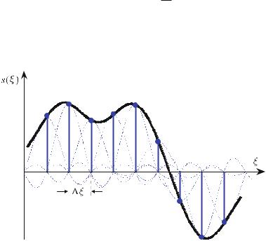
|
4 Fundamentals of Signal Processing |
If the frequency or spatial functions, originating from the convolution with the comb function, are free from any overlaps, the sampled function related by the Fourier transform can be reconstructed faultlessly.
At this point, an important question remaining is how to regain an analog signal from a sampled signal. For the reconstruction of the signal provided in Fig. . , lowpass filtering is necessary. An ideal low-pass filter
Hlp(u) = |
ξ rect |
u |
|
|
|
|
( . ) |
||
ξ |
|
|
|||||||
is a rectangular function of the height |
ξ inside |
the interval |
|
|
ξ , |
ξ , |
|||
|
|
|
[− ( |
|
) + ( |
)] |
|||
i.e., a multiplicative rectangular filter |
|
|
u |
|
|
||||
S(u) = Sa(u) ξ rect |
|
|
|
|
( . ) |
||||
ξ |
|
|
|
||||||
in the frequency domain. Referring to the convolution theorem ( . ), this expression can be represented in the spatial domain by a convolution
s(ξ) = sa(ξ) > sinc |
ξ |
. |
( . ) |
ξ |
This means that the signal recovery is a convolution of the sampling points with the sinc function. Figure . illustrates this principle, which is called the Shannon– Whittaker interpolation.
Fig. . . The sampled values of a spatially varying function are reconstructed by low-pass filtering the signal. The use of an ideal low-pass filter, which is represented by a rectangular filter in the frequency domain, corresponds to the convolution of the sampling points with the sinc function

4.19 Wiener–Khintchine Theorem |
|
For a deeper understanding, as well as more on the fundamental importance of the sampling theorem, the reader is referred to Lüke ( ). For further details on the Fourier transform of comb functions and the generalized boundary value for the solution of ( . ), the reader is referred to Klingen ( ) or Barrett and Swindell ( ).
4.19
Wiener–Khintchine Theorem
The Wiener–Khintchine theorem establishes a connection between the spatial variation of the signal, the amplitude spectrum, the autocorrelation function, and the energy density spectrum . Here, the Wiener–Khintchine theorem will be presented mathematically in two dimensions. This represents a good exercise for understanding its relation to the Fourier transform and the δ-distribution. Starting with the definition of the autocorrelation function of a general image f (x, y)
|
( |
|
+ + |
|
( |
|
) |
|
( |
|
+ |
|
+ |
|
) |
|
|
|
|
) =− − |
|
|
|
|
|
|
|
|
|||||||
C |
|
x, y |
∫ ∫ |
f |
|
ξ, η |
|
f |
|
x |
|
ξ, y |
|
η |
|
dξ dη , |
( . ) |
it can be shown via the inverse Fourier transform of the complex conjugate image, f (x, y), and the displaced image, f (x + ξ, y + η) respectively that the autocorrelation function is given by the inverse Fourier transform of the energy density spectrum. In Fig. . , the intermediate steps necessary for the derivation of the autocorrelation function via the Fourier transform are shown for the example of an abdominal image. First, the definition of the Fourier transform is incorporated as follows:
|
|
|
|
|
|
. |
|
|
|
|
|
|
|
|
|
|
|
|
|
|
|
|
|
|
|
|
|
|
|
|
|
. |
|
( |
|
+ + + − |
|
( |
|
|
|
|
|
) |
|
|
|
|
|
|
|
|
|
|
|
|
C |
||||||||
|
|
) =− − |
/− − |
F |
|
|
|
|
|
|
|
|
|
|
|
|
|
|
|
|
||||||||||||
C |
|
x, y |
∫ ∫ |
- ∫ ∫ |
|
|
u, v |
|
e−i π(u ξ+v η)du dvB |
|||||||||||||||||||||||
|
|
|
|
. |
+ .− |
|
|
|
|
|
|
|
|
|
|
|
|
|
|
|
|
|
|
|
|
|
|
|
|
. |
||
|
|
|
|
|
|
|
( |
|
|
|
) |
|
|
|
|
|
|
|
|
|
|
|
|
|
|
|
|
|
. |
|||
|
|
|
/− − |
|
|
|
|
|
i π |
u |
|
ξ |
x v |
η |
y |
|
C |
|||||||||||||||
|
|
|
|
- |
|
0 |
|
|
|
|
|
|
|
|
e |
( |
|
D |
||||||||||||||
|
|
|
|
∫ ∫ F u , v |
|
|
|
|
( |
|
|
|
+ )+ |
|
( |
+ |
))du dv B dξ dη . |
|||||||||||||||
|
|
|
|
. |
|
|
|
|
|
|
|
|
|
|
|
|
|
|
|
|
|
|
|
|
|
|
|
|
|
|
|
. |
The permutation |
of the integration order results in |
|
D |
|||||||||||||||||||||||||||||
0 |
|
. |
|
|
|
|
|
|
|
|
|
|
|
|
|
|
|
|
|
|
|
|
|
|
|
|
|
|||||
|
( |
|
+ + + − + − |
|
|
( |
|
|
|
) |
|
|
( |
|
|
|
) |
|||||||||||||||
|
|
) =− − |
/− − − − |
F |
|
|
|
|
|
u , v |
||||||||||||||||||||||
C |
|
x, y |
∫ ∫ |
- ∫ ∫ ∫ ∫ |
|
|
u, v |
|
F |
|
|
|||||||||||||||||||||
|
|
|
|
|
|
. |
|
|
|
|
|
|
|
|
|
|
|
|
|
|
|
|
|
|
|
|
|
|
|
|
|
. |
|
|
|
|
|
i π0u ξ |
|
|
|
|
|
|
|
|
|
|
|
|
|
|
|
|
|
|
|
|
|
|
|
|
|
||
|
|
|
|
|
v η |
|
i π |
|
|
u |
|
|
ξ |
|
x v |
η |
|
y |
|
|
|
|
|
C |
||||||||
|
|
|
|
e− |
( |
+ |
|
)e |
|
( |
|
|
|
( |
+ )+ |
|
( |
+ |
|
))du dv du dvB dξ dη . |
||||||||||||
|
|
|
|
|
|
|
|
|
|
|
|
|
|
|
|
|
|
|
|
|
|
|
|
|
|
|
|
|
|
|
|
. |
|
|
|
|
|
|
|
|
|
|
|
|
|
|
|
|
|
|
|
|
|
|
|
|
|
|
|
|
|
|
|
|
D |
( . )
( . )
To be precise, the following relation is the Wiener–Khintchine theorem only if f is a homogeneous and ergodic field (Jan ).
|
4 Fundamentals of Signal Processing |
Re-sorting the exponents
|
|
|
. |
|
|
|
|
|
|
|
|
( |
|
+ + + − + − |
|
( |
) |
( |
|
|
) |
||
|
) =− − |
/− − − − |
|
u |
, v |
||||||
C |
x, y |
∫ ∫ |
- |
∫ ∫ ∫ ∫ F |
|
|
u, v |
F |
|
||
|
|
|
. |
|
|
|
|
|
|
|
|
|
|
|
|
ei π(u0x+v y) ei π |
|
|
|
|
|
|
|
|
. |
||
|
|
|
|
|
|
|
|
|
|
|
C |
||||
|
|
|
|
(ξ(u −u)+η(v −v)) du dv du dvB dξ dη , |
|||||||||||
|
|
|
|
|
|
|
|
|
|
|
|
|
|
|
. |
and once again re-sorting the integration order, yields |
D |
||||||||||||||
|
( |
|
|
+ − + − |
|
( |
|
) |
|
( |
|
) |
|
|
|
|
|
) =− − − − |
|
|
|
|
|
|
|||||||
C |
|
x, y |
|
∫ ∫ ∫ ∫ F |
|
|
u, v |
|
F |
|
u , v |
|
ei π(u x+v |
y) |
|
|
|
|
|
. |
+ + |
|
|
|
|
|
|
|
|
. |
|
|
|
|
/− − |
|
|
|
|
|
|
|
|
C |
|
||
|
|
|
|
- |
∫ ∫ ei π(ξ(u −u)+η(v −v)) dξ dηB du dv du dv . |
||||||||||
|
|
|
|
. |
|
|
|
|
|
|
|
|
|
. |
|
|
|
|
|
0 |
|
|
|
|
|
|
|
|
|
D |
|
( . )
( . )
Due to property ( . ) the bracketed integral in the above equation is equivalent to a δ-distribution, giving
C(x, y)= ∫ ∫ ∫ ∫ F (u, v)F(u , v )ei π(u x+v y)δ(u −u, v −v)du dv du dv.
− − − −
( . )
Using the sifting property ( . ) of the δ-distribution it follows from ( . ), that
|
( |
|
|
|
|
+ − |
( |
|
|
|
) |
|
( |
|
|
) |
|
|
|
C |
x, y |
|
∫ |
∫ F |
u, v |
F |
u, v |
ei π(ux+v y) du dv |
( . ) |
||||||||||
|
|
|
|
) =− − |
|
|
|
|
|
|
|
|
|||||||
and therefore |
|
|
|
|
|
|
|
|
|
|
|
|
|
|
|
|
|
|
|
|
|
|
( |
|
|
) = |
+ − |
|
|
|
|
|
|
|
|
|
|
|
|
|
|
C |
x, y |
∫ ∫ |
|
F |
( |
u, v |
) |
ei π(ux+v y)du dv |
( . ) |
||||||||
or |
|
|
|
|
− − |
|
|
|
|
|
|
|
|
||||||
|
C(x, y) = F− F(u, v) = F− S(u, v) |
|
|||||||||||||||||
|
|
( . ) |
|||||||||||||||||
where S(u, v) is the energy density spectrum of the image f (x, y). |
|
||||||||||||||||||
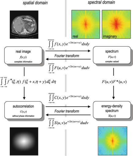
4.19 Wiener–Khintchine Theorem |
|
Fig. . . The Wiener–Khintchine theorem for image information. The corresponding transforms are given for an abdominal tomogram
The Wiener–Khintchine theorem is a special case of the general cross correla- |
|
tion function of two di erent images f (x, y) and g(x, y), for which |
|
Cfg(x, y) = F− F (u, v)G(u, v) |
( . ) |
holds. Result ( . ) is similar to the convolution theorem |
( . ). |

|
4 Fundamentals of Signal Processing |
4.20
Fourier Transform of Discrete Signals
Section . considered the Fourier transform of sampled signals. Considering the result in the one dimensional case,
|
( |
) = |
( |
) |
+ |
( |
|
− |
|
) A • ( |
|
) = |
|
|
+ |
|
|
|
− |
n |
|
|
sa |
|
ξ |
n ξ |
u |
|
|
|
S |
u |
|
( . ) |
|||||||||||
|
|
|||||||||||||||||||||
ξ |
|
s ξ |
|
n =− |
δ |
|
——— Sa |
|
ξ |
n =− |
|
|
ξ |
|
||||||||
|
|
|
|
|
|
|
|
|
|
|
|
|
|
|
|
|
|
|||||
has been obtained.
In this section the spectrum should be calculated directly by a Fourier transform of the sampled signal. The application of the Fourier transform to the left-hand side of ( . ) gives
|
|
+ |
|
|
+ |
|
|
|
|
|
|
|
|
( |
|
) =− |
( |
) |
( |
|
− |
|
|
) |
|
|
|
u |
|
ξ |
n |
ξ |
e−i πu ξ dξ . |
( . ) |
|||||||
Sa |
∫ |
s ξ |
|
n = − |
δ |
|
|
||||||
|
|
|
|
|
|
|
|
|
|
|
|
|
In ( . ) the function to be sampled can be moved inside the summation. Also, the order of the integration and the summation can be permuted, giving
( |
|
|
+ + |
( ) ( |
|
− |
|
|
) |
( . ) |
||||
u |
) =− |
|
|
ξ |
n ξ |
|||||||||
Sa |
|
∫ |
n |
= − |
s ξ δ |
|
|
|
|
e−i πu ξ dξ |
||||
|
|
|
|
|
|
|
|
|
|
|
|
|
||
|
|
= |
+ |
+ |
( ) ( |
|
|
− |
|
) |
|
|
||
|
|
|
− |
ξ |
n ξ |
e−i πu ξ dξ . |
||||||||
|
|
|
|
|
∫ |
s ξ δ |
|
|
|
|||||
|
|
|
n =− |
|
|
|
|
|
|
|
|
|
||
Using the sift property of the δ-distribution leads to
Sa(u) = |
+ |
|
s(n ξ)e−i πun ξ . |
( . ) |
n =−
As a result, the periodic spectrum only depends on the sampling values, s(n ξ). This transform is referred to as the discrete Fourier transform (DFT). In the literature, the sampling interval is sometimes set to ξ = (the unit of the sampling interval is therefore “one detector” or “one pixel”). In this case, the spectrum of the discrete signal s(n) is given by
|
( |
|
) = |
+ |
|
( |
|
) |
|
|
Sa |
u |
|
s |
n |
e−i πnu . |
( . ) |
||||
|
|
|
|
n =− |
|
|
|
|
|
|
( . ) is the complex notation of the Fourier series, so one may write
|
( |
|
) = |
+ |
|
|
Sa |
u |
|
sn e−i πun ξ , |
( . ) |
||
|
|
|
|
n =− |
|
|
where sn denotes the nth Fourier coe cient, which can be calculated by
|
|
|
sn = ξ ∫ξ |
Sa(u)ei πun ξ du . |
( . ) |
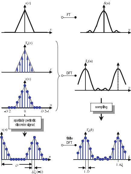
4.21 Finite Discrete Fourier Transform |
|
4.21
Finite Discrete Fourier Transform
In numerical calculations of the Fourier transform of discrete signals, only a finite number of frequencies must be calculated. Using the discrete Fourier transform, a discrete frequency spectrum is assigned to a discrete signal.
Fig. . . Relationship among the continuous signal, the sampled signal, and spatially limited and spatially discrete signals, as well as their respective spectra (adapted from Lüke [ ])

|
4 Fundamentals of Signal Processing |
If, as in the concrete case of a detector array in CT, the number of values of the discrete signal, s( ), s( ), . . . , s(D − ) , is limited to D, then, according to the sampling theorem, a sampling interval equal to the reciprocal length, D, of the detector array length is adequate (as mentioned above, the width of one detector element is set to ξ = ). The discrete sampled signal of the detector array, sa(n), which is periodic with period D, is assigned to the sampled spectrum, Sa(k). As shown above, the spectrum is also periodic. It follows that a calculation of D spectral values of one period is su cient. This is called the finite discrete Fourier transform (finite DFT). T he discrete frequency points are
uk = |
k |
for k = , . . . , D − |
( . ) |
D |
and the discrete frequency periodic Fourier transform of a spatially discrete, periodic signal within one period is
Sa |
( |
k |
) = |
D− |
sa |
( |
n |
) |
e−i πn Dk |
, |
( . ) |
|
|
|
|
|
|
|
|
|
|
||||
|
|
|
|
n = |
|
|
|
|
|
|
|
|
Table . . Classification of the Fourier transform. For each particular type, the table indicates
how the domain is being changed by the transform (the sampling length |
|
|
ξ is set to one) |
||||||||||||||||||||||||||||||||
|
|
|
|
|
|
|
|
|
|
|
|
|
|
|
|
|
|
|
|||||||||||||||||
|
|
|
|
Continuous space |
|
|
|
|
|
|
|
|
Discrete space |
|
|
|
|||||||||||||||||||
|
|
|
|
Fourier transform |
|
|
|
Discrete Fourier transform |
|||||||||||||||||||||||||||
|
|
|
|
|
|
Type: R R |
|
|
|
|
|
|
|
|
|
|
Type: Z [ , ] |
|
|
||||||||||||||||
Continuous |
|
|
|
|
+ |
|
|
|
|
|
|
|
|
|
|
|
|
|
|
|
|
|
+ |
|
|
|
|
|
|
|
|||||
( ) =− |
|
( ) |
|
|
|
|
|
|
|
|
|
|
|
|
|
|
|
|
( ) |
|
|
|
|
||||||||||||
|
|
|
−i πux |
|
|
|
|
( ) = n = |
|
|
−i πnu |
||||||||||||||||||||||||
frequency |
S u |
|
|
∫ s |
x |
|
e |
|
|
|
dx |
Sa |
|
u |
|
|
− s n e |
|
|
|
|||||||||||||||
|
|
|
|
|
|
|
|
|
|
|
|
|
|
|
|
|
|
|
|
|
|
|
|
|
|
|
|
|
|
|
|
|
|
|
|
|
|
|
|
|
|
Type: R R |
|
|
|
|
|
|
|
|
|
|
Type: [ , ] Z |
|
|
||||||||||||||||
|
|
|
( |
|
|
+ |
( ) |
|
|
|
|
|
|
|
|
( |
|
) = |
|
|
( ) |
|
|
|
|
|
|||||||||
|
|
|
|
) =− |
|
|
|
|
|
|
|
|
|
∫ |
|
|
|
|
|
|
|
||||||||||||||
|
|
s |
|
x |
|
|
∫ |
S u |
|
|
ei πux du |
s |
|
|
n |
|
|
|
Sa |
|
u |
ei πnu du |
|||||||||||||
|
|
|
|
|
|
Fourier series |
|
|
|
|
|
Discrete Fourier transform |
|||||||||||||||||||||||
|
|
|
|
|
Type: [ , D] Z |
|
|
|
|
|
|
|
|
Type: ZD ZD |
|
|
|||||||||||||||||||
Discrete |
|
( ) = |
|
|
|
D |
( ) |
|
|
|
|
|
|
|
|
|
|
|
|
D− |
|
|
( ) |
|
|
|
|
||||||||
|
|
|
|
|
|
|
|
|
|
|
( ) = n |
|
|
|
|
k |
|
||||||||||||||||||
frequency |
|
S k |
|
|
|
D |
∫ |
s x |
|
|
e |
D |
|
|
dx |
Sa |
|
k |
|
|
= |
sa n e |
|
|
D |
||||||||||
|
|
|
|
|
Type: Z [ , D] |
|
|
|
|
|
|
|
|
Type: ZD ZD |
|
|
|||||||||||||||||||
|
|
|
( ) = k |
|
|
( ) |
|
|
|
|
|
( ) = |
|
k |
( ) |
|
|
|
|||||||||||||||||
|
|
s x |
|
|
|
+ |
S k e |
ik |
π |
x |
sa n |
|
|
|
D− |
Sa k e |
i πn |
k |
|||||||||||||||||
|
|
|
|
|
|
|
|
|
D |
|
|
|
D |
|
|
|
|
D |
|||||||||||||||||
|
|
|
|
|
|
|
|
=− |
|
|
|
|
|
|
|
|
|
|
|
|
|
|
|
= |
|
|
|
|
|
|
|
||||

4.22 z-Transform
and the inverse transform is
sa |
|
|
D− |
|
i πn |
k |
|
|
|
n |
Sa k e |
D . |
( . ) |
||||||
D k = |
|
||||||||
|
( ) = |
|
|
( ) |
|
|
|
|
|
Figure . shows this relationship schematically. In summary, the transforms can be classified as shown in Table . .
4.22 z-Transform
The “z-transform” represents the generalization of the Fourier transform for spatially discrete signals. For a brief description of the z-transform and, subsequently, the “chirp z-transform”, the notation described here will follow that in Lüke ( ) and Stearns and Hush ( ).
The z-transform is used in cases where the discrete Fourier transform ( . ) does not converge for all series. This is the case if the sequence of the signal values, s(n), cannot be summed absolutely; therefore, the summation
|
= |
+ |
( |
|
) |
|
S |
|
n |
( . ) |
|||
|
|
n =− |
|
|
|
|
is not finite . In such cases, convergence can be achieved using a similar trick to the one that was used in ( . ). Convergence is assured by an exponential weighting, so that
|
|
|
|
|
|
|
|
|
|
|
+ |
( |
|
) |
|
|
|
< |
|
|
|
|
|
|
|
|||||||
|
|
|
|
|
|
|
|
|
|
|
|
|
n |
e−σn |
. |
|
|
|
|
|
( . ) |
|||||||||||
|
|
|
|
|
|
|
|
|
|
|
|
|
|
|
|
s |
|
|
|
|
|
|
|
|
|
|
||||||
|
|
|
|
|
|
|
|
|
|
n =− |
|
|
|
|
|
|
|
|
|
|
|
|
|
|
|
|
||||||
Then, the discrete Fourier transform according to ( . ) exists, so |
|
|||||||||||||||||||||||||||||||
|
( |
|
) |
|
A |
• |
+ |
|
( |
|
|
) |
|
|
|
|
|
|
|
|
= |
+ |
|
( |
|
) |
|
|
||||
s |
n |
e−σn |
|
s |
n |
e−σn e−i πnu |
|
s |
n |
e−(σ+i πu)n . |
( . ) |
|||||||||||||||||||||
|
|
——— |
n =− |
|
|
|
|
|
n =− |
|
|
|||||||||||||||||||||
|
|
|
|
|
|
|
|
|
|
|
|
|
|
|
|
|
|
|
|
|
|
|
|
|
|
|
|
|
||||
Thus, by substituting z |
= |
e(σ+i πu) |
|
|
right-hand side of ( . ) becomes |
|
||||||||||||||||||||||||||
|
|
|
|
|
|
|
|
|
|
( |
|
|
|
|
, the+ |
|
( |
|
|
) |
|
|
|
|
|
|
|
|
||||
|
|
|
|
|
|
|
|
|
S |
z |
) = |
|
|
s |
n |
z−n . |
|
|
|
|
|
( . ) |
||||||||||
|
|
|
|
|
|
|
|
|
|
|
|
|
|
|
|
|
|
|
|
|
|
|
||||||||||
n =−
( . ) is referred to as the z-transform. Decomposing the complex frequency variable into its absolute value and phase,
z = z eiφ = eσ ei πu |
( . ) |
Typically, delta impulses appear in the spectrum Sa(u).
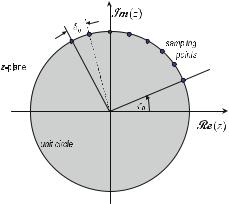
|
4 Fundamentals of Signal Processing |
allows the interpretation in the complex z-plane. In this plane, at each circle of radius
z = eσ , |
( . ) |
one period of the Fourier spectrum Sa(u) of the corresponding spatially discrete signal, s(n)e−σn , is located. This generalization of the Fourier transform includes a larger class of signals. The circular domain, in which the Fourier spectra converge, i.e., ( . ) is fulfilled, represents the region of convergence for the z-transform. For spatially limited signals the region of convergence covers the entire z-plane – with exception of the origin. If the region of convergence contains z = , then the Fourier and the z-transform are related to each other by the substitution z = ei πu (where σ = ). This means that the z-transform calculated over the unit circle is identical to the discrete Fourier transform (DFT). If the region of convergence does not contain the unit circle, the DFT is not defined for this series (Stearns and Hush ).
4.23
Chirp z-Transform
The chirp z-transform is an algorithm for the calculation of the z-transform of a series of finite length with sampling values in the frequency domain that are set at equal intervals along a generalized path in the z-plane (Stearns and Hush ). To preserve the reference to the Fourier transform, only paths representing arc sections of the unit circle are taken into account (cf. Fig. . ). The chirp z-transform will be important when considering the “linogram sampling” of the Radon space in Sect. . .
Fig. . . The chirp z-transform can be used to calculate M sampling values of the z-transform on the unit circle
4.23 Chirp z-Transform |
|
Let s(n) n= ,...,N− be a series of N sampled values in the spatial domain, whose spectrum is of interest. According to ( . ), the z-transform is then given by
|
( |
|
) = |
N− |
|
( |
|
) |
|
|
S |
z |
|
s |
n |
z−n . |
( . ) |
||||
|
|
|
|
n = |
|
|
|
|
|
|
Since in this case the z-transform is calculated over the unit circle by the substitution z = ei πu , it is identical to the discrete Fourier transform.
Consider the Fourier transform of M sampling values on the unit circle, starting from the angle φ and sampling at intervals of δ . The sampling along an arc can be described by
where |
|
|
|
|
|
zk = AB−k |
with k = , . . . , M − , |
|
|
|
|
|
|
|
|
|
( . ) |
|||||||||||||||||||||||||||||||||
Substituting into ( . ) givesA = eiφ |
|
and |
|
B = e−iδ . |
|
|
|
|
|
|
|
|
|
|
|
|
|
( . ) |
||||||||||||||||||||||||||||||||
|
N− |
( ) |
|
|
|
|
|
|
|
n |
= |
|
N− |
|
( ) |
|
|
|
|
|
|
|
|
|
|
|
|
= |
|
|
|
|
|
|
− |
|
|
|
||||||||||||
( ) = |
|
|
|
−k |
− |
|
|
|
|
|
|
|
−n |
|
nk |
|
|
|
|
|
|
|
|
|
|
|
|
|
|
|
||||||||||||||||||||
S z |
n = |
s n AB |
|
|
|
|
|
|
|
|
|
|
n = |
s n A |
|
|
B |
|
where k |
|
, . . . , M |
|
. |
( . ) |
||||||||||||||||||||||||||
|
|
|
|
|
|
|
|
|
|
|
|
|
|
|
|
|
|
|
|
|
|
|
|
|
|
|
|
|
|
|
|
|
|
|
|
|
|
|
|
|
|
|
|
|
||||||
The fact that (k−n) |
|
|
= k |
|
− kn+n |
|
, |
results in the Bluestein identity (Bluestein ) |
||||||||||||||||||||||||||||||||||||||||||
|
|
|
|
|
|
|
|
|
|
|
|
|
|
|
|
|
|
|
|
|
|
|
|
|
|
|
|
|
|
|
|
|||||||||||||||||||
|
|
|
|
|
|
|
|
|
|
|
kn = |
|
Pk |
|
|
+ n |
|
|
− (k − n) |
|
Q , |
|
|
|
|
|
|
|
|
|
|
( . ) |
||||||||||||||||||
|
|
|
|
|
|
|
|
|
|
|
|
|
|
|
|
|
|
|
|
|
|
|
|
|
|
|
||||||||||||||||||||||||
which, inserted into ( . ), gives the expression |
( ) |
|
|
|
|
|
|
|
|
|
|
|
|
|||||||||||||||||||||||||||||||||||||
( |
) = |
( ) |
|
|
|
|
|
n |
|
|
k |
|
|
|
|
(k−n) |
= |
|
|
k |
|
|
|
|
|
n |
|
|
(k−n) |
|
||||||||||||||||||||
|
N − |
|
|
−n |
|
|
|
|
|
|
|
− |
|
|
|
|
|
|
N − |
|
|
|
|
|
−n |
|
|
|
− |
|
||||||||||||||||||||
S zk |
n = |
s n A |
|
B |
|
|
|
B |
|
|
B |
|
|
|
|
|
|
|
|
|
|
|
B |
|
n = |
s n A |
B |
|
|
B |
|
|
|
|
|
. ( . ) |
||||||||||||||
|
|
|
|
|
|
|
|
|
|
|
|
|
|
|
|
|
|
|
|
|
|
|
|
|
|
|
|
|
|
|
|
|
|
|
|
|
|
|
|
|
|
|
|
|
|
|
||||
Furthermore, by replacing |
|
|
|
|
|
|
|
|
|
|
|
|
|
|
|
|
|
|
|
|
|
|
|
|
|
|
|
|
|
|
|
|
|
|
|
|
|
|
|
|
||||||||||
|
|
|
|
|
|
|
gn |
|
|
|
s n A−n B |
n |
|
and |
hn B− |
n |
, |
|
|
|
|
|
|
|
|
|
( . ) |
|||||||||||||||||||||||
|
|
|
|
|
|
|
|
|
|
|
|
|
|
|
|
|
|
|
|
|
|
|
||||||||||||||||||||||||||||
|
|
|
|
|
|
|
|
|
|
|
. ) becomes a linear convolution |
|
|
|
|
|
|
|
||||||||||||||||||||||||||||||||
the sum of products from (= |
|
|
( |
|
) |
|
|
|
|
|
|
|
|
|
|
|
|
|
|
|
= |
|
|
|
|
|
|
|
|
|
|
|
|
|
|
|
||||||||||||||
|
|
|
|
|
|
|
|
|
|
|
|
|
|
|
( |
|
|
|
) = |
|
|
|
k |
N − |
|
|
|
|
|
|
|
|
|
|
|
|
|
|
|
|
|
|
||||||||
|
|
|
|
|
|
|
|
|
|
|
|
|
|
|
|
|
|
|
|
|
|
|
|
|
|
|
|
|
|
|
|
|
|
|
|
|
|
|
|
|
|
|
|
|||||||
|
|
|
|
|
|
|
|
|
|
|
|
|
S |
zk |
|
B |
gn hk−n . |
|
|
|
|
|
|
|
|
|
|
|
|
( . ) |
||||||||||||||||||||
|
|
|
|
|
|
|
|
|
|
|
|
|
|
|
|
|
|
|
|
|
|
|
|
|
|
|
|
|
|
|
|
|
|
|||||||||||||||||
n =
With ( . ) the e orts pay back, because the convolution can be performed very e ciently in the Fourier domain by means of the fast Fourier transform (FFT).
The name “chirp” relates to the form of
|
= ein δ n , |
|
hn = eiδ n |
( . ) |
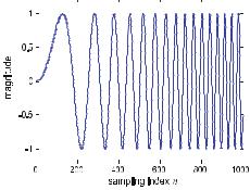
|
4 Fundamentals of Signal Processing |
||
|
|
|
|
|
|
|
|
Fig. . . Example of a chirp signal: The sinusoidal behavior of the signal’s imaginary part ( . ) with linearly increasing frequency
whose imaginary part is illustrated in Fig. . . hn is a complex oscillation with a linearly increasing frequency.

5Two-Dimensional Fourier-Based Reconstruction Methods
Contents
5.1 Introduction . . . . . . . . . . . . . . . . . . . . . . . . . . . . . . . . . . . . . . . . . . . . . . . . . . . . . . . 151 5.2 Radon Transformation . . . . . . . . . . . . . . . . . . . . . . . . . . . . . . . . . . . . . . . . . . . . . . . . 153
5.3 Inverse Radon Transformation and Fourier Slice Theorem . . . . . . . . . . . . . . . . . . . . . . 163
5.4 Implementation of the Direct Inverse Radon Transform . . . . . . . . . . . . . . . . . . . . . . . 167
5.5 Linogram Method . . . . . . . . . . . . . . . . . . . . . . . . . . . . . . . . . . . . . . . . . . . . . . . . . . . 170 5.6 Simple Backprojection . . . . . . . . . . . . . . . . . . . . . . . . . . . . . . . . . . . . . . . . . . . . . . . . 175 5.7 Filtered Backprojection . . . . . . . . . . . . . . . . . . . . . . . . . . . . . . . . . . . . . . . . . . . . . . . 179
5.8 Comparison Between Backprojection and Filtered Backprojection . . . . . . . . . . . . . . . . 183
5.9 Filtered Layergram: Deconvolution of the Simple Backprojection . . . . . . . . . . . . . . . . . 187
5.10 Filtered Backprojection and Radon’s Solution . . . . . . . . . . . . . . . . . . . . . . . . . . . . . . . 191
5.11 Cormack Transform . . . . . . . . . . . . . . . . . . . . . . . . . . . . . . . . . . . . . . . . . . . . . . . . . . 194
5.1 Introduction
On April the Austrian mathematician Johann Radon presented his work
On the Determination of Functions from their Integrals along Certain Manifolds at the annual meeting of the Royal Saxonian Society of Physical and Mathematical Sciences . The most important theorems of this work have been extracted and translated here using Radon’s own terminology to introduce the variables used throughout the subsequent chapters.
If one integrates a function of two variables (x, y) – a function f (x, y) in the plane – that satisfies suitable regularity conditions, along an arbitrary straight line L, then the values p(L) of these integrals define a line function.
Original German title: Über die Bestimmung von Funktionen durch ihre Integralwerte längs gewisser Mannigfaltigkeiten.
Physikalisch-Mathematische Königlich Sächsische Gesellschaft der Wissenschaften.
Translation by R. Lohner, School of Mathematics, Georgia Institute of Technology, Atlanta, GA, USA, first printed in Deans ( ).
|
5 Two-Dimensional Fourier-Based Reconstruction Methods |
The problem that is solved in this paper is the inversion of this linear functional transformation, i.e., answers to the following questions are given: Is every line function that satisfies suitable regularity conditions obtainable by this process? If this is the case, is the point function f then uniquely determined by p, and how can it be found?
Let f (x, y) be a real function defined for all real points r = [x, y] that satisfies the following regularity conditions:
a)f (x, y) is continuous.
b)The following double integral, which is to be taken over the whole plane, is convergent:
f (x,+y) dx dy . ( . ) x y
=[x, y] and any R : , let
|
|
|
|
|
|
|
r(R) = |
|
π |
f (x + R cos(γ), y + R sin(γ)) dγ . |
|
|
|
|
|
|||||||||||||||||
|
|
|
|
|
|
|
∫ |
|
|
( . ) |
||||||||||||||||||||||
|
|
|
|
|
|
f |
|
|
||||||||||||||||||||||||
|
|
|
|
|
|
π |
|
|
||||||||||||||||||||||||
Then for every point r, |
|
|
|
|
|
|
|
|
|
|
|
|
|
|
|
|
|
|
|
|||||||||||||
|
|
|
|
|
|
|
|
|
|
|
|
|
|
|
|
|
|
|
|
|
|
|
|
|
|
|||||||
|
|
|
|
|
|
|
|
|
|
|
|
|
|
lim |
f |
r |
|
R |
. |
|
|
|
|
|
|
|
( . ) |
|||||
|
|
|
|
|
|
|
|
|
|
|
|
|
|
R |
( ) = |
|
|
|
|
|
|
|
|
|
|
|
||||||
Thus the following theorems hold. |
|
|
|
|
|
|
|
|
|
|
|
|||||||||||||||||||||
Theorem I: The integral of f along the straight line L with the equation |
|
|
||||||||||||||||||||||||||||||
given by |
|
|
|
|
|
|
|
|
|
x cos(γ) + y sin(γ) = ξ , |
|
|
|
|
|
|
|
( . ) |
||||||||||||||
|
( |
|
) = |
|
(− |
|
+ |
|
|
+ |
( |
|
|
|
( |
|
) − |
( |
) |
|
( |
|
) + |
|
( |
|
)) |
|
||||
|
|
|
|
|
|
) =− |
|
|
|
|
|
|
|
|
|
|
||||||||||||||||
p |
|
ξ, γ |
|
p |
|
|
|
ξ, γ |
|
π |
|
∫ |
f |
|
ξ cos |
|
γ |
|
η sin γ |
|
, ξ sin |
|
γ |
|
η cos |
|
γ |
|
dη |
|||
( . )
is “in general” well defined. This means that on any circle those points that have tangent lines (see Fig. . – not given in Radon’s original paper) for which p does not exist form a set of linear measure zero.
Theorem II: If the mean value of p(ξ, γ) is formed for the tangent lines of the circle with center r = (x, y) and radius R:
pr(R) = |
π |
|
π ∫ p (x cos(γ) + y sin(γ) + R, γ) dγ , |
( . ) |
then this integral is absolutely convergent for all r = (x, y) and R. Theorem III: T he value of f(x, y) is completely determined by p and can be computed as follows:
f (r) = −π |
|
dprR(R) . |
|
∫ |
( . ) |
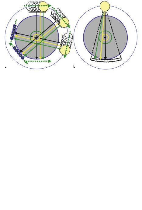
|
|
|
|
|
|
|
5.2 Radon Transformation |
|
|
|
|
|
|
|
|
|
|
|
|
|
|
|
|
|
|
|
|
|
|
|
|
|
|
|
|
Fig. . . a Due to the circular orbit of the X-ray source, the projection paths – visualized by the straight lines L on which the X-ray photons are running through the tissue – are organized as tangents of circles with an iso-center at point r = ( , ) inside the measurement field. b This circular sampling structure can be found in fan-beam geometry as well. In Sect. . the coordinate transformation between penciland fan-beam geometry will be discussed in detail
The following sections of this chapter will explain how Radon’s results can be understood in terms of modern computed tomography (CT). In particular, they demonstrate how the integral inversion is technically realized and in Chap. the practical aspects of the implementation are discussed in detail.
5.2
Radon Transformation
Today, CT systems use fan-beam geometry . However, it is more instructive to introduce CT reconstruction by describing those methods that use pencil geometry, in which, for every direction of projection, the X-ray beam is collimated to a pencil shape and moved linearly in the direction parallel to a linear X-ray detector array. This concept has already been mentioned in Sect. . with regard to the first generation of CT systems. Sequentially, the X-ray sampling unit is rotated by an angle γ, and, subsequently, moved linearly. This process is repeated until any point of the object to be reconstructed is illuminated by at least . Figure . shows this sampling process schematically.
The three-dimensional extension of the fan-beam concept to cone-beam geometry will be discussed in Chap. .
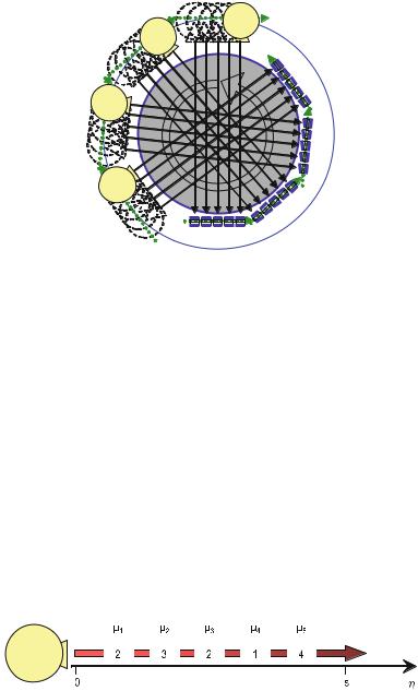
|
5 Two-Dimensional Fourier-Based Reconstruction Methods |
Fig. . . Schematic drawing of pencilor needle-beam geometry in first-generation CT systems. The X-ray beam, confined to a pencil or needle shape by collimation, produces a parallel projection via a parallel shift of the X-ray tube in the direction parallel to the linear detector array for any projection angle. The sectional plane defined by this projection geometry is the tomographic slice that is to be reconstructed
For a fixed projection angle γ and a particular linear shift position of the X-ray source, one is interested in the projection integral
p(s) = |
s |
|
∫ μ(η)dη . |
( . ) |
If the attenuation coe cient changes in discrete steps only, as Fig. . suggests, one obtains the projection sum
|
( |
s |
|
|
|
p |
) = |
μk |
η |
( . ) |
|
s |
k = |
||||
|
|
|
|
|
instead of the projection integral of ( . ).
Note that, since the X-ray source is moved parallel to the X-ray detector array, the integration length s used in ( . ) and ( . ) is constant.
Fig. . . Attenuation of the radiation intensity when passing through inhomogeneous tissue. Due to the inhomogeneity of the attenuation coe cients along the integration length, the values cannot be reconstructed by a simple inversion. However, the e ort required by the reconstruction is paid back, since exactly this spatial distribution of attenuation coe cients forms the image of clinical interest
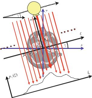
5.2 Radon Transformation |
|
On the other hand, there are a number of parallel paths through the object, which define a sectional plane or CT slice. Therefore, it is sensible to write the projection integral as a function of the linear position of the source – or the location of the corresponding detector element, ξ – and the projection angle γ, and no longer as a function of the constant path s between X-ray tube and detector element. For this purpose, a coordinate system (ξ, η) is defined, which rotates on the gantry together with the X-ray source and the detector. This coordinate system will be referred to as the rotating sampling system – in contrast to the fixed patient coordinate system (x, y). Figure . visualizes the correspondence between the two coordinate systems.
By a repetition of the alternating rotation and shifting sequence of the rigidly connected source-detector system – often referred to as rotating disk on the gantry – a set of parallel projections pγ (ξ), pγ (ξ), pγ (ξ), . . . is measured, from which the spatial distribution of the object points or, more precisely, the spatial distribution of the attenuation coe cients within a selected slice of the patient, has to be reconstructed. In Fig. . an axial cranial tomography is used as an example to demonstrate the correspondence of the coordinate systems that will be used extensively throughout this chapter.
Fig. . . The sampling disk rotating on the gantry of the tomograph carries the X-ray tube and the detector. When both elements are shifted synchronously and parallel to each other for any angle γ, the X-rays parallel to each other in the rotating sampling system (ξ, η) define the slice that is to be reconstructed. Here, as an example, this slice is axial cranial tomography
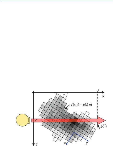
5 Two-Dimensional Fourier-Based Reconstruction Methods
In this special case of constant integration length, s, the projection integral |
|
under projection angle γ defined in the rotating (ξ, η) system, is written as |
|
s |
|
pγ (ξ) = ∫ μ(ξ, η)dη . |
( . ) |
Figure . visualizes the projection integral for the passage of X-ray photons through the tissue. In practice, the spatial distribution of the attenuation coe cients that are to be reconstructed is a discrete set of values only. This is obviously due to the limited resolution of the real sampling, displaying, and storing system. However, in this chapter signals are assumed to be continuous. This again allows a more instructive introduction to the theory of image reconstruction. The reconstruction procedures being implemented in the field are actually based on discrete signals and will be discussed in detail in Chap. .
( . ) represents an integration along the path of the traveling photons given by the position ξ of the X-ray source and the X-ray detector respectively under a certain projection angle γ. In practice, one is not interested in expressing the attenuation values, μ, as a function of the rotating sampling system (ξ, η). In fact, the image of the spatial distribution of attenuation values must be given as a function of the fixed
Fig. . . The object is seen to rotate if viewed from a point traveling with the X-ray tube in the (ξ, η) frame. The spatial distribution of the reconstructed attenuation coe cients is a discrete set of values in the actual measuring situation
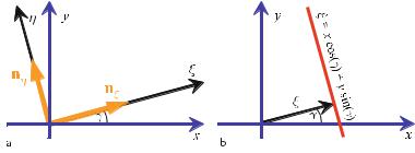
|
|
|
|
|
|
|
|
|
|
|
5.2 |
Radon Transformation |
|
patient coordinate system x, y . To describe the relation between the coordinate |
|
||||||||||||
|
in a first step the unit vectors |
|
|
||||||||||
systems (ξ, η) and (x, y), ( |
) |
|
|
|
= |
cos |
γ |
|
|
|
|
||
and |
|
|
nξ |
( ) |
|
|
( . ) |
|
|||||
|
|
|
|
|
sin(γ) |
|
|
|
|||||
|
|
|
|
|
|
|
|
sin |
γ |
|
|
|
|
|
|
nη = −cos((γ)) |
|
( . ) |
|
||||||||
are defined. These vectors span the rotating |
ξ, η |
|
frame. Figure . visualizes the |
|
|||||||||
|
|
|
|
|
|
|
|
|
rotating sampling disk on the gantry |
|
|||
rotating unit vectors that are attached to the( |
) |
|
|
|
|||||||||
and the patient at rest in the fixed |
|
x, y |
|
system. |
|
|
|
|
|||||
|
To describe the projection |
path – and along with that the projection integral |
|
||||||||||
|
|
|
( |
|
|
) |
|
|
|
|
|
|
|
( . ) – in the fixed patient coordinate system the geometric relations |
|
||||||||||||
and |
ξ = rT ċ nξ = x cos(γ) + y sin(γ) |
( . ) |
|
||||||||||
|
η = rT ċ nη = −x sin(γ) + y cos(γ) |
( . ) |
|
||||||||||
are given between the two coordinate systems for a particular point within the object to be imaged, r = (x, y)T. With the help of ( . ) and ( . ), the variables of the attenuation coe cient in ( . ) can be substituted such that
f (x, y) = μ (ξ(x, y), η(x, y))
= μ rT ċ nξ , rT ċ nη
Fig. . . a Definition of the rotating sampling system (ξ, η) by unit vectors. The fixed (x, y) coordinate system represents the patient coordinate system at rest. b A projection line through the object can be given in terms of the Hessian normal form
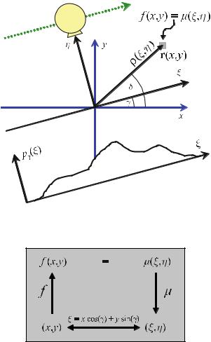
|
5 Two-Dimensional Fourier-Based Reconstruction Methods |
expresses the attenuation values f in the fixed (x, y) system. From a physical point of view, f and μ are identical attenuation coe cients for the tissue at the point r = (x, y)T in the fixed (x, y) system and at the point ρ = (ξ, η)T in the rotating (ξ, η) system. In Fig. . this relation is schematically shown.
The relation of the attenuation coe cients in the rotating sampling and the fixed patient system is summarized in the functional chart in Fig. . .
Fig. . . The attenuation coe cients f at the point r in the fixed (x, y) patient system and μ at the point ρ in the rotating (ξ, η) sampling system
Fig. . . Functional correspondence of the attenuation coe cients defined in the fixed (x, y) and the rotating (ξ, η) coordinate system
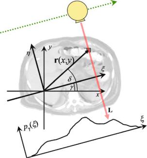
5.2 Radon Transformation |
|
From the view point of signal processing, the stepwise shift of the X-ray source represents a sampling process of a continuous projection signal. Let L be a δ-line in the sectional plane, the sampling can then be described as follows
f > δ(L) = R∫ |
f (r)δ(r − L)dr |
( . ) |
|
or, equivalent by |
|
|
|
f > δ(L) =r ∫L |
f (r)dr . |
( . ) |
|
Figure . shows the sampling process in a plane, again schematically. The line L is the set of all points in the tissue that is to be examined. Since L is the path of X-ray photons for a certain position (ξ, γ) of the X-ray tube, the meaning of ( . ) or ( . ) is that all attenuation values in the tissue along the line L are integrated. In fact, this reflects the physical process of X-ray attenuation by matter.
Fig. . . Line sampling of the object. All points of the tissue lying on the line L are passed through by X-ray photons. The resulting exponential decay of the X-ray intensity is due to the attenuation values lying on the line L
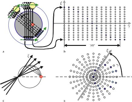
|
5 Two-Dimensional Fourier-Based Reconstruction Methods |
Due to the sifting property of the δ-distribution ( . ) results in the sum of all points r of the sectional plane that lie on line L. Since the physical interpretation of the line L is the X-ray photon path, L may be substituted by (rTnξ) = ξ, because ξ is the detector position for counting the remaining photons. The projection integral ( . ) can thus be written as follows
f |
> |
δ |
( |
L |
) = |
∫ |
f |
( |
r |
) |
δ |
(( |
rT |
ċ |
nξ |
) − |
ξ |
) |
dr |
|
|
||
|
|
|
|
|
|
|
|
|
|
|
|
|
|||||||||||
|
|
|
|
|
|
|
|
|
( |
|
) ( |
|
( ) + |
( ) − ) |
|
||||||||
|
|
|
|
|
|
=− − |
|
|
|
( . ) |
|||||||||||||
|
|
|
|
|
|
|
∫ |
|
∫ |
|
f |
|
|
x, y |
δ x cos γ |
y sin γ ξ dx dy |
|
||||||
|
|
|
|
|
|
|
p |
ξ . |
|
|
|
|
|
|
|
|
|
|
|
|
|
||
As mentioned above |
the projections vary with the projection angle γ. Therefore, the |
||||||||||||||||||||||
= ( ) |
|
|
|
|
|
|
|
|
|
|
|
|
|
|
|||||||||
parameter γ must be included in a complete description of the projection process: p = p(ξ, γ) = pγ (ξ) . ( . )
Fig. . . a Arrangement of the measured projection values pγ(ξ). Projection data are usually displayed in a Cartesian (ξ, γ) grid. Such a Radon space diagram is often called a sinogram. Note that the sinogram is related to the data space of a Hough transformation (see Lehmann et al. [ ]). Occasionally, one also uses a polar coordinate grid (d) to visualize Radon space data (b). The circles in the polar arrangement of the projection values stem from the theorem of Thales (c)
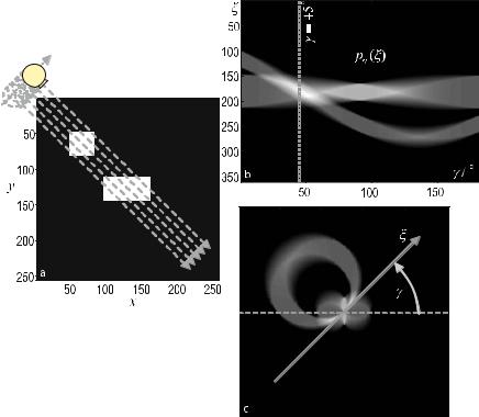
5.2 Radon Transformation |
|
pγ (ξ) is called the two-dimensional Radon transform of the object. One may write
or |
( ) A R |
|
• > ( ) = |
γ ( ) |
|
f |
x, y ——— f δ L |
p ξ |
( . ) |
||
|
pγ (ξ) = R f (x, y) |
|
( . ) |
||
respectively. A detailed discussion of the properties of the Radon transform can be found in Helgason ( ).
Figure . schematically shows a diagram of Radon-transformed data. Typically, the projection values pγ (ξ) of the Radon space are arranged in a Cartesian (ξ, γ) diagram. In such a diagram, the projection values of objects that lie outside the rotation center of the tomograph produce a sinusoidal trace. Therefore, this graphical representation of projection values is often called a sinogram. Figure . shows the formation of the sinusoidal curve for a single object point.
Fig. . . a Synthetic pixel image. The homogeneous attenuation values of two objects are simulated by gray values set to . b Cartesian Radon space of the synthetic image provided in a. c Radon space of the synthetic image in polar coordinates
|
5 |
|
Two-Dimensional Fourier-Based Reconstruction Methods |
||||||||
|
|
|
|
Projection data are acquired from to only, since, according to the phys- |
|||||||
|
ical symmetry, the X-ray path back through the object that is to be examined pro- |
||||||||||
|
vides no additional information to the forward path. Figure . a shows a synthetic |
||||||||||
|
tomogram with an homogeneous square shifted away from the rotation center and |
||||||||||
|
an homogeneous rectangle at the rotation center. Figures . b and c display the |
||||||||||
|
Radon space corresponding to Fig. . a. In the diagram the projection values pγ ξ |
||||||||||
|
|
|
|
|
|
|
|
|
|
|
and |
|
are displayed in gray values. High integral attenuation is represented by white ( ) |
||||||||||
|
low attenuation by black. Figure . a shows the projection values in the Cartesian |
||||||||||
|
|
ξ, γ plane. The sinusoidal trace of the projection values in the Radon space for |
|||||||||
|
the square in the object space can be easily recognized. The further an object is |
||||||||||
|
( |
|
) |
|
|
|
|
|
|
||
|
apart from the rotation center the larger is the modulation amplitude of the corres- |
||||||||||
|
ponding sine trace in the Radon space. The rectangle therefore does not show this |
||||||||||
|
global sinusoidal path. Nevertheless, the rectangular shape can be identified due |
||||||||||
|
to the characteristic path of the values in the Radon space as well. Under a view of |
||||||||||
|
γ the rectangle and the square lie on the same line according to the projection |
||||||||||
|
geometry. This situation, indicated by the dashed line in Fig. . b, is reflected by an |
||||||||||
|
|
= |
|
|
|
|
|
( |
|
|
|
|
exceedingly high value at p |
. |
|||||||||
|
|
|
|
|
|
|
|
) |
|
|
|
|
|
|
|
|
|
|
|
|
|
|
|
|
|
|
|
|
|
|
|
|
|
|
|
|
|
|
|
|
|
|
|
|
|
|
|
|
|
|
|
|
|
|
|
|
|
|
|
|
|
|
|
|
|
|
|
|
|
|
|
Fig. . . a Computed tomographic slice image of the abdomen. b Cartesian Radon space of the abdomen provided in a. c Radon space of the abdomen provided in a in polar coordinates

5.3 Inverse Radon Transformation and Fourier Slice Theorem |
|
Figure . c shows the Radon space in polar coordinates. Both object representations are well separated from each other. The further an object is apart from the rotation center the larger the corresponding circle in the polar Radon space. For the rectangle in the center of Fig. . a the mirror symmetrical nature in the object space leads to a mirror symmetric signature in the Radon space. The pattern of the polar Radon space representation is a result of the theorem of Thales (Papula ).
As an example, Fig. . a shows a tomographic slice of an abdomen. Figure . b and c again represent the corresponding Radon space. The interpretation of these diagrams is more complicated, as in the case of the synthetic tomogram, since each point of the object produces its own sinusoidal trace of di erent amplitude, phase, and gray value. However, this data set represents the basis for the following reconstruction methods.
5.3
Inverse Radon Transformation and Fourier Slice Theorem
( . ) presents a first important result. However, in practice one faces the inverse problem already formulated by Johann Radon in . One is interested in the spatial distribution of attenuation values f (x, y) = μ(ξ, η), having measured only the projection data pγ (ξ). The Fourier slice theorem that is summarized in Scheme . does indeed solve this problem. It is divided into three main steps.
While steps and can be directly carried out by the simple application of the Fourier and the inverse Fourier transforms respectively, step requires knowledge of a certain identity of the Fourier transforms of f (x, y) and pγ (ξ). To understand this identity, in a first step the Radon space data p(ξ, γ) = pγ (ξ) are seen as onedimensional functions of the detector coordinate ξ parameterized by the projection angle γ. This means that for every projection angle γ a one-dimensional spectrum
|
( |
|
) = |
|
( |
|
|
|
( |
|
) |
|
|
|
|
|
|
) =− |
|
|
|
|
|||||
P |
|
q, γ |
|
Pγ |
|
q |
∫ |
pγ |
|
ξ |
|
e− πiq ξ dξ |
( . ) |
Scheme . Fourier slice theorem
. Calculation of the Fourier transform of pγ (ξ)
pγ (ξ) −−−−−−−−−• Pγ (q)
. Construction of the Fourier transform of f from P Pγ (q)•−−−−−−−−−• F(u, v)
. Calculation of the inverse Fourier transform of F provides the desired function f F(u, v)•−−−−−−−−− f (x, y)
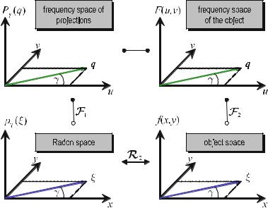
|
5 Two-Dimensional Fourier-Based Reconstruction Methods |
|
|
|
|
|
|
is obtained. This transformation completes step of Scheme . . To carry out step |
|||||
|
one has to keep in mind that F is a function of the Cartesian spectral coordinates u |
|||||
|
and v, because the spatial distribution of attenuation coe cients f |
|
x, y |
|
is defined |
|
|
in Cartesian coordinates as well. The transformation into a |
spectral representation |
||||
|
|
( |
|
) |
|
|
|
does not change the nature of the coordinate system, which means |
|
|
|
||
|
F(u, v) •———A f (x, y) . |
|
|
|
|
( . ) |
Using an inverse two-dimensional Fourier transform, this step can also be carried out easily.
If, however, the Fourier transform does not change the nature of the coordinate system, it is obvious that a change in coordinates has to be carried out in step , because the Radon transform pγ (ξ), along with its Fourier transform Pγ (q), are given in polar coordinates (ξ, γ) and (q, γ) respectively. Figure . shows this relation schematically. The transformations in the vertical direction of Fig. . are given by the Fourier transform in each case. However, from left to right a change in coordinates from polar to Cartesian coordinates has to be carried out.
As shown in Fig. . , the spatial vector ξ = ξ(ξ, γ) points in the same direction as the spectral vector q = q(q, γ). This is due to the rotational variance of the Fourier transform.
Fig. . . Schematic representation of the Fourier slice theorem. Since the Fourier transform does not change the nature of coordinate systems, a change from polar to Cartesian coordinates has to be carried out to find the correspondence between F(u, v) and Pγ (q). T he polar nature of the Radon space is inherently produced by the circular sampling of the Cartesian object space
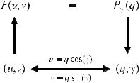
5.3 Inverse Radon Transformation and Fourier Slice Theorem |
|
To change the coordinate systems it is briefly repeated here that a point with the polar coordinates (q, γ) has the Cartesian coordinates
u = q cos(γ) v = q sin(γ) .
When replacing the Cartesian coordinates with polar coordinates of the function F(u, v) on the left-hand side of transformation ( . ), one obtains
F (u(q, γ), v(q, γ)) = F (q cos(γ), q sin(γ))
= Fpolar(q, γ) .
The Fourier slice theorem ensures that Fpolar(q, γ) is identical to Pγ (q), thus
F (q cos(γ), q sin(γ)) = P(q, γ) = Pγ (q) .
This means that a linear radial intersection of the two-dimensional Fourier spectrum F(u, v) of the spatial distribution of attenuation values f (x, y) at angle γ equals the one-dimensional Fourier transform Pγ (q) of the measured Radon values pγ (ξ) that result from the projection of f under the angle γ. Figure . shows this important relation schematically in a functional diagram.
The functional relation shown in Fig. . can be derived directly from the coordinate transformation rules. Starting with
Pγ (q) = |
|
|
∫ pγ (ξ)e− πiq ξ dξ , |
( . ) |
−
it must be recalled that the projection values pγ (ξ) in ( . ) result from the projection integral ( . ), such that
|
|
|
|
. |
|
|
|
|
|
. |
|
|
( |
|
) =− |
/ |
∫ |
|
( |
|
) |
C |
|
Pγ |
|
q |
∫ |
- |
μ |
|
ξ, η |
|
dηB e− πiq ξ dξ . |
( . ) |
|
|
|
|
|
. |
|
|
|
|
|
. |
|
|
|
|
|
0 |
|
|
|
|
|
D |
|
|
|
|
|
|
|
|
|
|
|
|
|
Fig. . . Schematic functional presentation of the Fourier slice theorem identity. In the spectral representation F(u, v) and Pγ (q) can be identified with each other if a change in coordinates from Cartesian to polar coordinates is carried out
|
5 Two-Dimensional Fourier-Based Reconstruction Methods |
The integration in the direction of the X-ray path through the object, i.e., the inner term of ( . ), can be extended to infinity, if one assumes that outside the object to be examined no attenuation occurs. Hence,
|
( |
|
( |
|
) |
|
|
|
) =− − |
|
|
|
|||
Pγ |
q |
∫ ∫ |
μ |
ξ, η |
|
e− πiq ξ dξ dη . |
( . ) |
As a next step, the coordinate system has to be changed from the rotating sampling system (ξ, η) to the patient system (x, y) at rest. Both systems are of Cartesian nature. Thus, the integration element, dξ dη, can be directly replaced with dx dy, such that
|
|
( |
|
|
|
|
|
|
( |
|
( |
|
|
|
) |
|
( |
|
)) |
|
|
||
|
|
|
) =− − |
|
|
|
|
|
|
|
|
|
|||||||||||
|
Pγ |
|
q |
|
|
∫ ∫ |
μ |
|
ξ |
|
x, y |
|
, η |
|
x, y |
|
e− πiq(rT ċnξ ) dx dy . |
( . ) |
|||||
The inner product |
|
rTnξ |
|
|
ξ, introduced in ( . ), in the exponent of ( . ) also |
||||||||||||||||||
includes the |
transition to the fixed |
x, y |
system. With the correspondence repre- |
||||||||||||||||||||
|
|
|
( |
|
|
|
) = |
|
|
|
|
|
( ) |
|
|
|
|
|
|||||
sented by ( . ) it follows that |
|
|
|
|
|
|
|
|
|
||||||||||||||
|
|
|
|
|
|
( |
|
|
|
|
|
( |
|
|
) |
|
|
|
|
||||
|
|
|
|
|
|
|
|
) =− − |
|
|
|
|
|
|
|
||||||||
|
|
|
|
|
Pγ |
|
q |
|
∫ ∫ |
|
f |
|
x, y |
|
e− πiq(rTċnξ ) dx dy . |
( . ) |
|||||||
To prove that ( . ) is identical to the two-dimensional Fourier transform of the object, one starts with the Cartesian formulation of the Fourier transform of the tomographic section f (x, y) in the fixed patient coordinate system
|
( |
|
|
|
( |
|
) |
|
|
|
|
) =− − |
|
|
|
|
|||
F |
|
u, v |
∫ ∫ |
f |
|
x, y |
|
e− πi(xu+yv) dx dy . |
( . ) |
Inserting the polar relations from ( . ) in the exponent of ( . ) one obtains
|
( |
|
|
|
( |
|
) |
|
|
|
|
) =− − |
|
|
|
|
|||
F |
|
u, v |
∫ ∫ |
f |
|
x, y |
|
e− πi(x q cos(γ)+yq sin(γ))dx dy . |
( . ) |
After factoring out the radial frequency variable q in the exponent, ( . ) simplifies to
|
( |
|
|
|
( |
|
) |
|
|
|
|
) =− − |
|
|
|
|
|||
F |
|
u, v |
∫ ∫ |
f |
|
x, y |
|
e− πiq rTċnξ dx dy |
( . ) |
through substitution of ( . ). The integrand in ( . ) is identical to the one in ( . ), whereby it is shown that
F |
( |
u, v |
u=q cos(γ) |
= |
Pγ |
( |
q |
) |
. |
( . ) |
|
|
) v=q sin(γ) |
|
|
|
|
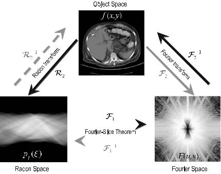
|
|
5.4 Implementation of the Direct Inverse Radon Transform |
|
||||||||||
|
|
|
|
|
|
|
|
|
|
|
|
|
|
|
|
|
|
|
|
|
|
|
|
|
|
|
|
|
|
|
|
|
|
|
|
|
|
|
|
|
|
|
|
|
|
|
|
|
|
|
|
|
|
|
|
|
|
|
|
|
|
|
|
|
|
|
|
|
|
|
|
|
|
|
|
|
|
|
|
|
|
|
|
|
|
|
|
|
|
|
|
|
|
|
|
|
|
|
|
|
|
|
|
|
|
|
|
|
|
|
|
|
|
|
|
|
|
|
|
|
|
|
|
|
|
|
|
|
|
|
|
|
|
|
|
|
|
|
|
Fig. . . Schematic summary of the relations among the spatial object domain (shown as an axial abdomen tomogram), the Radon space (given over an interval of from the object), and the Fourier space (only absolute values are shown). The Fourier domain results directly from the spatial domain by a two-dimensional Fourier transform of the object, but can also be obtained by the Fourier slice theorem using a set of one-dimensional Fourier transforms of the projection profiles in the Radon space
This is a core result of the Fourier slice theorem and the most important result for all Fourier-based reconstruction methods. ( . ) can also be used in the reverse direction to give a Radon transform when the image f (x, y) is known. Figure . summarizes the relation among the spatial domain of the object, the Radon space, and the Fourier space of both. The Fourier slice theorem can be expressed in one sentence. It states that the one-dimensional Fourier transform of the projection profile can be identified with a radial line in the Cartesian Fourier space of the object drawn at the angle of the corresponding measurement.
5.4
Implementation of the Direct Inverse Radon Transform
Using the main result of the Fourier slice theorem stated by ( . ), a simple direct algorithmic scheme for tomographic object reconstruction f (x, y) from the measured projection data pγ (ξ) can be given. In such a scheme the polar spectral data
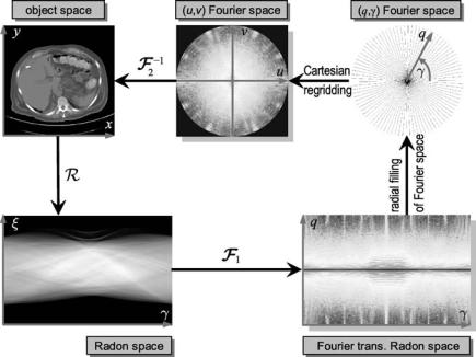
|
5 |
|
|
|
Two-Dimensional Fourier-Based Reconstruction Methods |
|
|
|
|
|
|
|
|
|
|
|
||||||||||||||
|
Pγ |
( |
q |
) |
of the projections have to be sorted into a spectral Cartesian coordinate sys- |
|||||||||||||||||||||||||
|
|
|
|
|||||||||||||||||||||||||||
|
tem (u, v . In this way, the function F u, v is assembled. An inverse Fourier trans- |
|||||||||||||||||||||||||||||
|
form of F) u, v |
back into the spatial |
domain directly leads to the desired tomogram |
|||||||||||||||||||||||||||
|
( |
) |
|
|
|
|
|
|
|
|
|
|
|
|
|
|
|
|||||||||||||
|
|
( |
|
|
|
) |
Figure . shows the direct reconstruction scheme as a flow chart. |
|
|
|
|
|||||||||||||||||||
|
f x, y . |
( |
|
) |
|
|
|
|
|
|
|
|
|
|
|
|
|
|
|
|
|
|
|
|||||||
|
|
|
|
|
Unfortunately, there is a practical di culty one is faced with the simple direct |
|||||||||||||||||||||||||
|
inverse Radon transform. Due to data handling problems and dose considerations, |
|||||||||||||||||||||||||||||
|
a CT scanner is obviously limited with regard to the number of projections |
|
pγ |
|
ξ , |
|||||||||||||||||||||||||
|
p |
|
|
( ) |
|
|
|
|
( ) |
|
|
|
|
|
|
|
|
|
|
sampling |
||||||||||
|
|
γ |
|
ξ , . . . , pγN |
|
ξ that can be measured within one revolution of the |
|
|
|
|
( ) |
|||||||||||||||||||
|
disk. Therefore, the values of the Fourier transform F u, v |
|
of the attenuation co- |
|||||||||||||||||||||||||||
|
e cients f |
|
x, y are only known for a limited |
number of measured radial lines in |
||||||||||||||||||||||||||
|
|
|
|
|
( |
) |
|
|
|
|
|
|
|
|
|
|||||||||||||||
|
|
|
|
|
( |
|
) |
space. |
|
|
|
|
|
|
|
|
|
|
|
|
|
|
|
|
|
|
||||
|
the |
|
|
u, v |
|
|
( |
|
) |
|
|
|
|
|
|
|
|
|
|
|
|
|
|
|
|
|
||||
|
|
|
|
|
The sampling discretization of the projection angle γ itself, however, is not the |
|||||||||||||||||||||||||
|
problem. The problem lies in the position, or more precisely, the distribution of the |
|||||||||||||||||||||||||||||
|
polar spectral data in the Cartesian coordinate system. The spectral representation |
|||||||||||||||||||||||||||||
|
of the tomographic spatial domain is only known on radial, “star-like” lines. |
|
|
|
|
|||||||||||||||||||||||||
|
|
|
|
|
Figure . a shows the radial configuration of the Fourier transform Pγ q |
|
of |
|||||||||||||||||||||||
|
the projection data measured at angle γ |
in the Cartesian |
|
u, v space. |
Obviously, |
|||||||||||||||||||||||||
|
|
|
|
|
|
( |
) |
|
||||||||||||||||||||||
|
the spectral projection data lie on circles in the |
u, v |
|
space. Since the fast Fourier |
||||||||||||||||||||||||||
|
|
|
( |
|
) |
|
|
|
|
|
|
|
|
|||||||||||||||||
|
|
|
|
|
|
|
|
|
|
|
|
|
|
|
|
rectangular grid, the data P |
|
q , |
||||||||||||
|
transform (FFT) needs data lying on a regular( |
|
) |
|
|
|
|
|
|
|
|
γ |
|
|||||||||||||||||
|
which are arranged in circles, must be defined on a Cartesian grid before |
inverse |
||||||||||||||||||||||||||||
|
|
|
( |
|
) |
|||||||||||||||||||||||||
transformation. This process is called regridding.
Fig. . . Flow chart of the direct reconstruction scheme based on the Fourier slice theorem
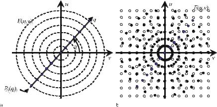
|
|
|
|
|
5.4 Implementation of the Direct Inverse Radon Transform |
|
|||
|
|
|
|
|
|
|
|
|
|
|
|
|
|
|
|
|
|
|
|
|
|
|
|
|
|
|
|
|
|
|
|
|
|
|
|
|
|
|
|
|
|
|
|
|
|
|
|
|
|
|
|
|
|
|
|
|
|
|
|
|
|
|
|
|
|
|
|
|
|
Fig. . . a Radially arranged values Pγ (q)obtained from the one-dimensional Fourier transform of projection measurements. b Regridding of the spectral projection data, initially being arranged in a polar coordinate frame, onto a Cartesian grid. The radial and the Cartesian sample points of the spectral data of Pγ (q) and F(u, v) only lie directly above each other on the u and v axes that span the Fourier space of the object
In order to perform the direct inverse Radon transformation using an FFT algorithm, the Cartesian grid has to be created from the polar configuration of spectral data via an appropriate interpolation (e.g., nearest-neighbor, bilinear, etc.). As a direct consequence of the radial data arrangement – as illustrated in Fig. . b – the density of measured spectral data in the (u, v) space decreases for higher frequencies. Therefore, the interpolation error increases at high spatial frequencies. Unfortunately, this e ect leads to a degradation of image quality because high spatial frequencies represent image areas that are rich in detail.
As a counter-measure, the geometrical sampling may be changed in order to obtain those projection values in the Radon space that lie exactly on a Cartesian grid in the Fourier space of the object. Due to the fact that the Radon space and Fourier space are connected via the Fourier transform, the complementary variables ξ and q behave reciprocally to each other, i.e., when the sampling points in the Radon space are arranged on concentric circles (see Fig. . a), the sampling points in the corresponding Fourier space (see Fig. . b) lie on circles as well, and vice versa. Obviously, this is due to the fact that the sampling points in the Radon space are equidistant in all radial directions.
If, on the other hand, the points in the Fourier space are expected to lie on a Cartesian grid, this has consequences for the required locations of the sampling points in the Radon space. Looking at Fig. . d it can be seen that the Fourier points are located on the boundary of concentric squares. Since in the spectral domain the sampling points on the diagonals of these squares have greater separation than the sampling points on the u and v axes, the quadratic shape is not preserved by the inverse Fourier transform back into Radon space. Due to the reciprocal relation
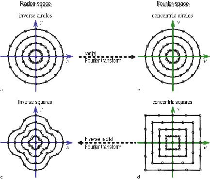
|
5 Two-Dimensional Fourier-Based Reconstruction Methods |
||||
|
|
|
|
|
|
|
|
|
|
|
|
|
|
|
|
|
|
Fig. . . a Radially arranged values of pγ(ξ) obtained from projection measurements are lying on concentric circles. b After the radial Fourier transform, the values of Pγ (q) are lying on concentric circles as well. c Arrangement of sampling points in the Radon space on inverse concentric squares consisting of four semi-circles. d Regular arrangement of points on concentric quadrants in the Fourier space
between Fourier and Radon space variables, the sampling points on the diagonals in the Radon space must lie closer to each other than the corresponding points on the x- and y-axes. One obtains what is called “inverse squares” as visualized in Fig. . c. The formation of inverse squares during the measurement process by the linogram method will be discussed in the following section.
5.5
Linogram Method
One way to overcome the problem of two-dimensional interpolation when using the direct inverse Radon transform is called the “linogram method” (Jacobson ; Magnusson ). As motivated by the discussion in the previous section, spectral sampling points on concentric squares in the Fourier space are created instead

5.5 Linogram Method |
|
of concentric circles by a sophisticated non-equidistant sampling procedure. The inverse chirp z-transform (Stearns and Hush ; cf. Sect. . ) is optimally adapted to this very situation such that no interpolation is necessary.
The linogram method can be seen as a direct Fourier method. However, instead of the sinogram sampling arrangement of the projection data introduced above, here a slightly di erent data structure, namely a linogram, has to be created or measured. For this linogram sampling arrangement, the overall sampling length b varies with the projection angle γ such that
|
( |
|
) = & |
b |
( |
|
cos γ |
for |
|
|
|
γ |
|
|
|
||
b |
γ |
|
|
|
) ( ) |
|
|
|
|
|
< |
|
|
( . ) |
|||
|
|
|
|
b( |
|
)sin (γ ) |
for |
|
|
γ |
|
. |
|
||||
|
|
|
|
|
− |
|
|
|
|
< |
|
|
|||||
b( ) represents the overall sampling length for the projection angle γ = . Figure . shows the corresponding sampling points, for an exemplary projection angle for each of the two intervals given by ( . ). The detector arrays that are fixed for this kind of sampling arrangement (drawn in bold in Fig. . for each case of ( . )) coincide with the x- and y-axes respectively of the fixed patient coordinate system. For comparison, the rotating detector array of the sinogram sampling arrangement is also shown.
Fig. . . Linogram sampling a in the angle interval − γ < and b in the angle interval γ < . The sampling points are indicated on virtual fixed detector lines in each case (see the bold x-axis in a and the bold y-axis in b). Obviously, the sampled overall length b(γ) has its minimum at
b( ) = D ξ similar to the sinogram sampling arrangement, where D is the number of sampling points.
|
5 Two-Dimensional Fourier-Based Reconstruction Methods |
|||||||
|
|
|
|
|
|
|
|
|
|
|
|
|
|
|
|
|
|
|
|
|
|
|
|
|
|
|
|
|
|
|
|
|
|
|
|
|
|
|
|
|
|
|
|
|
|
|
|
|
|
|
|
|
|
Fig. . . For linogram sampling, two circles are the underlying shapes that confine the length of the radial sampling line. The circles can be constructed with the theorem of Thales for each of the angle intervals a − γ < and b γ < . c Overall, a Radon space sampling point confinement is established by four semi-circles
For a fixed distance between the sampling points on the linear detector array, it is obvious that the overall length b(γ) that is actually sampled, has its minima at the projection angles γ = and γ = , and its maxima at γ = and γ = respectively. When the projection angle γ is varied, the length b(γ) draws a circle according to the theorem of Thales. In this way, two circles are the underlying shape of data arrangement in the Radon space domain for each of the two angle intervals, as presented in Fig. . .
Overall, the allowed sampling area in the Radon space is defined by four semicircles that are constructed with the theorem of Thales for each of the two angle intervals given by ( . ). The reciprocal relation between the Radon space and the Fourier space has already been mentioned above. If an overall length b has been sampled in the Radon space, a sampling point distance of b− is the consequence in the Fourier space. Since the number of sampling points D is not altered by the Fourier transform, the corresponding overall length of the radial Fourier transform B must change when the projection angle is varied. Obviously, the overall length in the Fourier space B(γ) has its maxima at the projection
|
|
|
|
|
|
|
|
|
|
|
|
|
|
|
|
|
|
|
|
|
|
|
|
5.5 Linogram Method |
|
|
angles γ |
= |
|
|
|
|
|
|
|
|
|
|
|
|
|
|
|
|
= |
|
|
|
|
|
|
||
ively. |
|
and γ |
= , and its minima at γ |
|
|
|
and γ = respect- |
|
||||||||||||||||||
The Fourier space length is given by |
|
|
|
|
|
|
|
|
|
|
|
|
|
|||||||||||||
|
|
|
|
|
|
- |
|
|
|
D |
|
|
|
|
|
for − |
γ < |
|
|
|||||||
|
|
|
B |
( |
γ |
b |
|
cos γ |
|
|
( . ) |
|
||||||||||||||
|
|
|
|
|
) = / |
( |
|
)D |
( |
|
) |
|
|
|
|
|
|
|
|
|
|
|
||||
|
|
|
|
|
|
. |
|
|
|
for |
|
γ |
< |
|
|
|
|
|||||||||
|
|
|
|
|
|
|
|
|
|
) |
|
|
|
|||||||||||||
|
|
|
|
|
|
0 |
|
( |
|
) |
sin |
( |
γ |
|
|
|
|
|
|
|
|
|
||||
|
|
|
|
|
|
. b |
|
|
|
|
|
|
|
|
|
|
|
|
|
|
||||||
as a direct consequence of ( . ). |
|
|
|
|
|
|
|
|
|
|
|
|
|
|
|
|
|
|||||||||
( . ) leads to concentric sampling areas with a quadratic form in the Fourier |
|
|||||||||||||||||||||||||
space. In this way, the spectral sampling points in the |
u, v |
space are arranged |
|
|||||||||||||||||||||||
on horizontal and vertical lines, as required. However, |
the distribution of sampling |
|
||||||||||||||||||||||||
|
( |
|
|
) |
|
|
||||||||||||||||||||
points on the boundaries of the Fourier space squares does not completely solve |
|
|||||||||||||||||||||||||
the interpolation problem. Along the horizontal and vertical lines of the sampling |
|
|||||||||||||||||||||||||
directions given by the Fourier space squares, equidistant sampling points can be |
|
|||||||||||||||||||||||||
achieved when choosing a non-constant projection angle increment, |
γ. In fact, |
|
||||||||||||||||||||||||
equidistant sampling points in the spectral domain are obtained by choosing con- |
|
|||||||||||||||||||||||||
stant increments for |
|
|
tan(γ) for |
− γ < |
|
|
|
|
|
|
||||||||||||||||
and |
|
|
|
|
|
|
|
|
|
( . ) |
|
|||||||||||||||
|
|
|
|
|
|
cot(γ) for γ < |
|
|
|
|
|
|
||||||||||||||
|
|
|
|
|
|
|
|
|
|
|
( . ) |
|
||||||||||||||
respectively. This results directly from the geometry of the squares in the Fourier space. Figure . a and b summarize the linogram method schematically. According to the segmentation into the angle intervals − γ < and γ < during the linogram-based data acquisition in the Radon space, these areas can be treated separately and fitted together in a later step. After separation of the angle intervals, a radial Fourier transform is applied that leads to the desired equidistant vertical arrangement of points for the interval − γ < and the equidistant horizontal arrangement for the interval γ < .
The sampling point density in the Fourier space is inhomogeneous, i.e., the density of spectral sampling points increases for decreasing spatial frequencies. This over-representation of slowly varying object information is compensated for by a linear weighting of the frequency space. Since the inverse chirp-z transform treats all points with the same weight, an uncompensated transformation would have the e ect of a low-pass filtering.
Hereafter, the inverse chirp-z transform is applied in the vertical direction for the angle interval − γ < and in the horizontal direction for the comple-
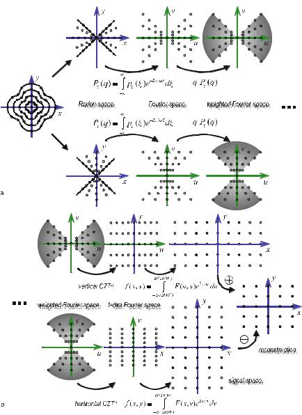
|
5 Two-Dimensional Fourier-Based Reconstruction Methods |
|||||||||||||||||||||||
|
|
|
|
|
|
|
|
|
|
|
|
|
|
|
|
|
|
|
|
|
|
|
|
|
|
|
|
|
|
|
|
|
|
|
|
|
|
|
|
|
|
|
|
|
|
|
|
|
|
|
|
|
|
|
|
|
|
|
|
|
|
|
|
|
|
|
|
|
|
|
|
|
|
|
|
|
|
|
|
|
|
|
|
|
|
|
|
|
|
|
|
|
|
|
|
|
|
|
|
|
|
|
|
|
|
|
|
|
|
|
|
|
|
|
|
|
|
|
|
|
|
|
|
|
|
|
|
|
|
|
|
|
|
|
|
|
|
|
|
|
|
|
|
|
|
|
|
|
|
|
|
|
|
|
|
|
|
|
|
|
|
|
|
|
|
|
|
|
|
|
|
|
|
|
|
|
|
|
|
|
|
|
|
|
|
|
|
|
|
|
|
|
|
|
|
|
|
|
|
|
|
|
|
|
|
|
|
|
|
|
|
|
|
|
|
|
|
|
|
|
|
|
|
|
|
|
|
|
|
|
|
|
|
|
|
|
|
|
|
|
|
|
|
|
|
|
|
|
|
|
|
|
|
|
|
|
|
|
|
|
|
|
|
|
|
|
|
|
|
|
|
|
|
|
|
|
|
|
|
|
|
|
|
|
|
|
|
|
|
|
|
|
|
|
|
|
|
|
|
|
|
|
|
|
|
|
|
|
|
|
|
|
|
|
|
|
|
|
|
|
|
|
|
|
Fig. . a,b. Schematic presentation of the linogram-based reconstruction method
ment angle interval γ < . This results in frequency representation along the relevant directions such that a heterogeneous space of mixed spatial and spectral coordinates is produced for each case.
5.6 Simple Backprojection |
|
Along the spectral direction of this space, another one-dimensional inverse Fourier transform is applied, i.e.,
|
|
|
|
|
|
|
|
|
D |
|
|
|
|
|
|
|
|
|
|
|
|
|
|
|
|
|
|
|
|
|
|
|
|||
|
|
( |
|
|
|
|
|
b( ) |
|
|
( |
|
|
) |
|
|
|
− |
|
|
|
|
|
< |
|
|
|||||||||
|
|
|
|
) =− b(D ) |
|
|
|
|
|
|
|
|
|
|
|
|
|
||||||||||||||||||
f |
|
|
x, y |
|
|
|
∫ |
F |
|
|
u, y |
|
|
e πiux du |
for |
|
|
|
|
|
γ |
|
|
|
( . ) |
||||||||||
and |
|
|
|
|
|
|
|
|
|
|
|
|
|
|
|
|
|
|
|
|
|
|
|
|
|
|
|
|
|
|
|
|
|
|
|
|
|
|
|
|
|
|
|
|
D |
|
|
|
|
|
|
|
|
|
|
|
|
|
|
|
|
|
|
|
|
|
|
|
|||
|
( |
|
|
) =− |
|
b( ) |
|
|
( |
|
|
) |
|
|
|
− |
|
|
|
|
|
< |
|
|
|
||||||||||
|
|
|
b(D ) |
|
|
|
|
|
|
|
|
|
|
|
|
|
|||||||||||||||||||
f |
|
|
x, y |
|
|
|
|
∫ |
|
F |
|
|
x, v |
|
|
e πiv y dv |
for |
|
|
|
|
|
γ |
|
|
. |
( . ) |
||||||||
Each of the separately treated angle intervals leads to a separate image in the signal space of the object, which consists of only half of all projections. Finally, the complete reconstruction is obtained by adding the partial reconstructions f and f
f (x, y) = f (x, y) + f (x, y) . ( . )
Note that only mutually overlapping areas lead to the desired image. For a more detailed discussion of the linogram method, the reader is referred to C. Jacobson and M. Magnusson-Seger (Jacobson ; Magnusson ).
5.6
Simple Backprojection
As discussed above, the Fourier slice theorem induces a general direct reconstruction procedure. Having measured projections at an adequately high number of angles such that the spectral (u, v) space can be filled densely with data points, a simple inverse two-dimensional Fourier transform has to be applied to reconstruct the attenuation values, f (x, y), of the object. However, due to the abovementioned problems of Cartesian regridding, a di erent reconstruction strategy for sinogram data sampling is used in practice. In fact, today, all modern CT systems implement “filtered backprojection”.
To understand what the term filtered means in this context, let us step back for a moment. At first glance, one might think that the image that is to be reconstructed could potentially be obtained by a simple backprojection of the measured projection profiles pγ (ξ), just as suggested in Fig. . . Such a strategy would smear back the profile values in the direction from which the radiation came.
Mathematically, this process can be modeled by the following equation
π
g(x, y) = ∫ pγ (ξ)dγ
π
( . )
= ∫ pγ (x cos(γ) + y sin(γ))dγ .
|
5 Two-Dimensional Fourier-Based Reconstruction Methods |
|
|
|
|
|
|
|
||||
|
Although this kind of simple backprojection intuitively seems to reverse the process |
|||||||||||
|
of projection, the procedure does not result in the desired distribution of attenu- |
|||||||||||
|
ation values. In fact, the backprojection defined by ( . ) is not an adequate recon- |
|||||||||||
|
struction method for the original morphology of the objects in the image f |
|
x, y , |
|||||||||
|
because each point in the image grid receives non-negative contributions |
from all |
||||||||||
|
|
( |
) |
|||||||||
|
other points of the original image. This problem becomes immediately clear when |
|||||||||||
|
discussing the reconstruction of all points outside the support of the image, i.e., all |
|||||||||||
|
points f |
( |
x, y |
) = |
. Due to the fact that the projection profile pγ |
( |
ξ |
) |
is a non-negative |
|||
|
|
|
|
|
||||||||
function, the simple backprojection smears back non-negative values over the entire image. In this way, positive values are assigned to image pixels even outside the object. The backprojections from other directions cannot compensate for this incorrect pixel entry, because the entire set of projection profiles in the sinogram is a set of non-negative functions.
Looking at the backprojection process in detail by substituting ( . ) or ( . ) into ( . ), it follows that
g(x, y) =
=
=
|
π |
|
∫ ∫∫ f (r)drdγ |
|
|
|
all r L |
|
|
π |
|
∫ ∫∫ f (r)δ(r − L)drdγ |
( . ) |
|
r R
π
∫∫∫ f (r)δ (rT ċ nξ) − ξ drdγ .
r R
The line L, on which the backprojection takes place, can again be substituted by the Hessian normal form (r T ċ nξ) = ξ and by taking advantage of the δ-distribution symmetry
g(x, y) = |
π |
f (r )δ rT ċ nξ − r T ċ nξ dr dγ |
|
∫ r ∫∫R |
( . ) |
is obtained. Changing the order of integration in ( . ) results in
|
( |
|
) = |
|
|
( |
|
) |
π |
( |
|
− |
|
) |
|
ċ |
|
|
# |
|
|
|
|
|
∫ δ |
|
|
|
|
|
|||||||||||
g |
|
x, y |
r |
∫∫R |
f |
|
r |
|
|
r |
|
r |
|
T |
|
nξ |
|
dγ! dr . |
( . ) |
As indicated in Fig. . , let φ be the angle between the di erence vector (r − r ) and the x-axis.
In this way the inner product of (r − r ) and nξ in ( . ) can be replaced by
|
( |
|
) = |
|
|
|
( |
|
) |
π |
|
( |
|
− |
|
|
|
( |
|
− |
|
)) |
|
# |
|
|
g |
|
x, y |
|
∫∫ |
f |
|
r |
|
∫ |
δ |
|
r |
|
r |
|
cos |
|
φ |
|
γ |
|
dγ |
! |
dr . |
( . ) |
|
|
|
|
r |
|
R |
|
|
|
|
|
|
|
|
|
|
|
|
|
|
|
|
|
|
|
||
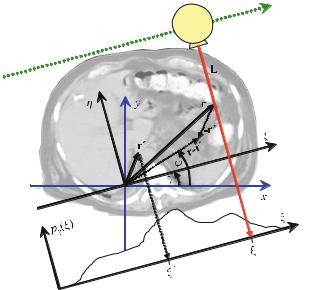
|
|
|
|
5.6 Simple Backprojection |
|
|
|
|
|
|
|
|
|
|
|
|
|
|
|
|
|
|
|
|
|
|
|
|
|
Fig. . . Reconstruction geometry for simple backprojection
When applying the rule ( . ) for calculations using the δ-distribution of functions, one obtains
|
|
|
r |
|
R |
|
|
|
|
|
r r( |
− ) |
|
|
! |
|
|
|||
|
( |
|
) = |
|
|
|
( |
|
) |
π |
S − |
SS |
|
$ |
|
S |
|
# |
|
|
g |
|
x, y |
|
∫∫ |
f |
|
r |
|
∫ |
δ γ γ |
π |
|
dγ |
|
dr |
( . ) |
||||
|
|
|
|
|
|
|
|
|
|
|
|
|
sin |
|
|
|
|
|
|
|
for the inner integral, since the argument of the δ-distribution is the functionr − r cos(φ − γ) of which the only zero value, γ , lies in the interval γ < π at γ = (φ −γ) = π (or −π , as the sign depends on φ). The denominator of the inner integral in ( . ) is constant in terms of integration along the projection angle, γ. The integration of the δ-distribution in the numerator results in the value , so that
( |
) =r R |
( ) r r |
|
|
||||||
g x, y |
|
∫∫ f r |
|
dr |
|
|||||
|
− |
( . ) |
||||||||
|
= |
+ + |
( |
|
|
|||||
|
− − |
|
|
|
) (x − x , y − y ) |
|
||||
|
|
∫ ∫ |
f |
|
x |
, y |
|
|
|
dx dy |
is obtained.
Obviously, ( . ) represents a convolution of the original image the function
h(x, y) = (x, y)
and thus,
g(x, y) = f (x, y) > h(x, y).
f (x, y) with
( . )
( . )
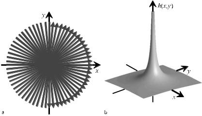
5.7 Filtered Backprojection |
|
As an aside, this result can also be found in electrodynamics, where the electric field around a very thin and infinitely long straight conductor decreases by r. In three-dimensional space the density of electric field lines around a point charge decreases by r . This decrease along with the distance is known from Coulomb’s law.
One might think that ( . ) represents a sensible reconstruction method, because in Fig. . the original point of the object can be detected as the maximum value in the image g(x, y). However, one has to keep in mind that any point of the object to be reconstructed is blurred by h(x, y). It will be shown later that the convolution of the image with the PSF results in an overall unacceptable blurring of the image. In fact, adequate reconstruction strategies can be found that include a suitable deconvolution of the image, thus compensating for the blurring e ects seen in naive backprojection.
5.7
Filtered Backprojection
What went wrong with the simple backprojection introduced in the previous section? To answer this question one has to focus on the Fourier slice theorem again. The identities of the Fourier transform of the desired image F(u, v) and the Fourier transform of the measured projections Pγ (q) have been shown in Sect. . . Since Pγ (q) is found as a radial line along the q-axis under the polar angle γ in the Cartesian (u, v) space, it is reasonable to have a closer look at the change from Cartesian to polar coordinates.
In fact, an image reconstruction procedure – the filtered backprojection – can be derived as a clever result of the coordinate transformation. As a first step to obtaining the image f (x, y) from projections, the inverse Fourier transform
f (x, y) = |
|
|
∫ ∫ F(u, v)e πi(xu+yv)du dv |
( . ) |
− −
applied to F(u, v) must be expressed in polar coordinates. To do this one substitutes
u = q cos(γ) v = q sin(γ) .
The infinitesimal area integration element du dv in ( . ) is transformed to J dq dγ, where J is the Jacobian, i.e.,
|
|
|
|
∂u |
|
|
∂v |
|
|
|
|
|
|
|
|
J |
det |
∂ u, v |
|
∂q |
|
|
∂q |
|
cos |
γ |
sin γ |
|
|||
|
|
|
|
|
|
|
|||||||||
∂(q, γ) |
|
∂u |
|
|
∂v |
|
|
q |
sin γ |
q cos γ |
( . ) |
||||
|
|
|
|
|
|
|
|||||||||
|
|
= |
|
|
|
|
|
( ) |
|
( ) |
|||||
( ) |
|
|
|
= 9 |
− |
|
|
( ) |
|
( )9 |
|
||||
∂γ ∂γ |
|
|
|
|
|||||||||||
|
|
|
= Hq cos (γH) + sin (γ) = q . |
|
|
||||||||||
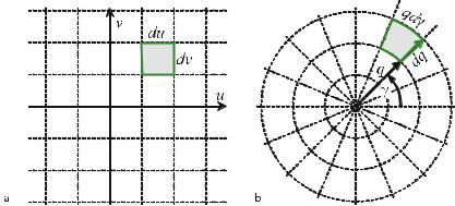
|
5 Two-Dimensional Fourier-Based Reconstruction Methods |
In Fig. . the use of the Jacobian is demonstrated. The area elements du dv, which must cover the entire two-dimensional plane in ( . ), have the same square shape, independent of their actual location in the plane (compare Fig. . a). However, it can be seen in Fig. . b that in polar coordinates the “tiles” q dq dγ change their shape as a function of distance from the origin.
When using the new infinitesimal mosaic of integration elements q dq dγ for the entire two-dimensional plane being described in polar coordinates, the inverse Fourier transform is given as
f (x, y) = ∫ ∫ F (q cos(γ), q sin(γ)) e πiq(x cos(γ)+y sin(γ))q dq dγ . ( . )
The outer integral in ( . ) can be split into two parts when treating the projections for the angles γ = [ , π] and γ = [π, π] separately. In this way one obtains
f (x, y) = |
π |
+ |
|
|
∫ |
∫ |
F(q, γ)e πiq(x cos(γ)+y sin(γ))q dq dγ |
( . ) |
|
|
+ |
π + |
|
|
|
∫ |
∫ F(q, γ)e πiq(x cos(γ)+y sin(γ))q dq dγ . |
|
|
|
|
π |
|
|
The π-shift of the angle interval in the second integral term with respect to the first term can be expressed by a phase shift of the functional terms, such that
f (x, y) = |
π |
+ |
|
|
|
|
|
|||
∫ |
∫ |
|
F(q, γ)e πiq(x cos(γ)+y sin(γ))q dq dγ |
( . ) |
||||||
|
+ |
π |
+ |
|
|
|
|
|
||
|
∫ |
∫ F(q, γ + π)e πiq(x cos(γ+π)+y sin(γ+π))q dq dγ . |
|
|||||||
|
|
|
|
|
|
|
|
|
|
|
|
|
|
|
|
|
|
|
|
|
|
|
|
|
|
|
|
|
|
|
|
|
|
|
|
|
|
|
|
|
|
|
|
|
|
|
|
|
|
|
|
|
|
|
Fig. . . Shape of the infinitesimal area integration elements in a Cartesian and b polar Fourier coordinates
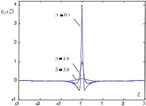
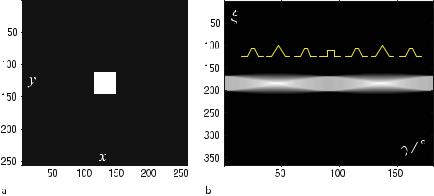
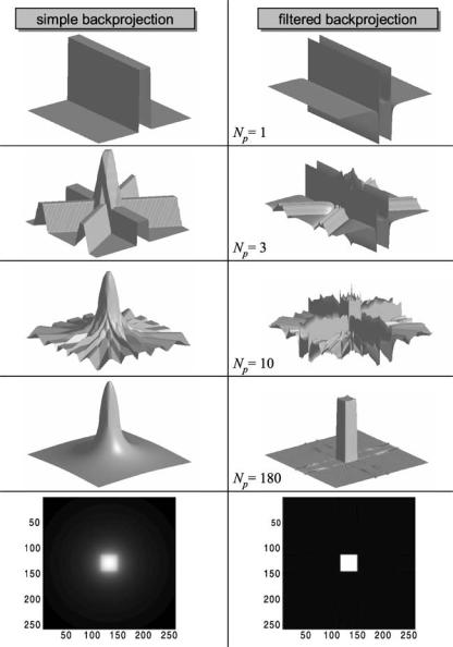
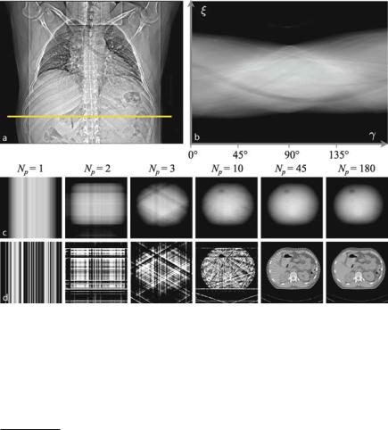


5.9 Filtered Layergram: Deconvolution of the Simple Backprojection |
|
This is the same expression as in Sect. . , ( . ) and leads to the Hankel transform, so that
|
|
+ π |
|
|
|
|
|
|
+ |
|
|
|
H(q) = H M |
|
|
|
|
|
|
|
|
|
|
|
|
|
O = ∫ |
∫ |
e−i πqr cos(γ)dγ dr |
= π ∫ |
J ( πqr)dr . |
( . ) |
||||||
r |
||||||||||||
With the substitution z = πqr it follows that |
+ |
|
|
|
||||||||
|
|
|
|
|
|
O = |
|
|
|
|
|
|
|
|
H(q) = H M |
|
|
∫ J (z)dz . |
( . ) |
||||||
|
|
r |
q |
|||||||||
After Abramowitz and Stegun ( ), the integral of the Bessel function of th order in ( . ) is
|
|
|
|
|
|
+ |
|
|
|
= |
|
|
|
|
|
|
||||
such that |
|
|
|
|
|
∫ J (z)dz |
|
|
|
|
|
( . ) |
||||||||
|
|
|
|
|
|
|
|
|
|
|
|
|
|
|
|
|
|
|
|
|
|
|
|
|
|
|
|
|
|
|
|
|
|
|
|
|
|
|
|
|
|
|
|
|
|
H(q) = H M |
|
O = |
q |
= |
6 |
|
|
|
. |
|
|
( . ) |
||||
|
|
|
|
r |
|
|
|
|||||||||||||
|
|
|
|
u |
+ |
v |
|
|
||||||||||||
Substituting this result into ( . ), it follows that |
|
|
|
|
|
|||||||||||||||
|
|
|
|
|
G(u, v) = F(u, v) |
|
|
|
|
|
|
|
||||||||
|
|
|
|
|
q . |
|
|
|
|
|
( . ) |
|||||||||
In this way, the deconvolution of the blurred image g |
x, y can be described as |
|||||||||||||||||||
|
( |
|
) = |
|
|
( |
|
|
|
) = |
|
|
|
|
|
( |
) |
|
|
|
f |
|
x, y |
|
F− |
q G |
|
u, v |
|
F |
− |
q F( |
|
g) x, y |
|
. |
( . ) |
||||
Scheme . Filtered layergram
. Calculation of the backprojection and integration over
π
g(x, y) = ∫ pγ (ξ)dγ
. Two-dimensional Fourier transform of the simple backprojection g(x, y) −−−−−−−−−•G(u, v)
. Multiplication of the Fourier transform with the distance to the origin and two-
dimensional inverse Fourier transform into the spatial domain |
|
u + v G(u, v)•−−−−−−−−− f (x, y) |
( . ) |
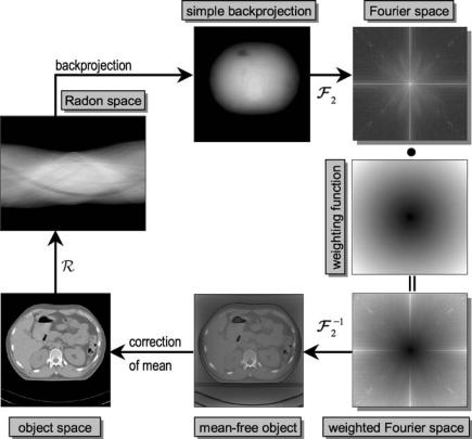
|
5 Two-Dimensional Fourier-Based Reconstruction Methods |
Fig. . . Exemplary illustration of the filtered layergram process. When starting from the Radon space and creating a simple backprojection g(x, y), the original image f (x, y) is obtained by: Weighting the Fourier transform G(u, v) of the simple backprojection with the distance function q in the frequency space; transforming it back to the spatial domain; and correcting the mean value of the image. The last step is necessary as the mean value of the image disappears by the distance weighting with q so that negative image values occur for the background
Obviously, the deconvolution filter q in ( . ) is a cone-shaped weighting function in the two-dimensional spectral domain. Since g(x, y) has been obtained by “smearing” back the unfiltered projections – see ( . ) – that are accumulated layerwise over , the reconstruction follows Scheme . , which is named a filtered layergram. Figure . illustrates the entire filtered layergram process exemplarily by means of an abdomen tomogram.
Please note that filtered backprojection and a filtered layergram are mathematically equivalent. However, in practice only filtered backprojection is implemented. This is due to the fact that the filtered backprojection reconstruction process can be started directly after measurement of the first projection profile. In this way, the re-
5.10 Filtered Backprojection and Radon’s Solution |
|
construction with filtered backprojection is faster, as data acquisition and image reconstruction can be performed almost simultaneously. The filtered layergram process needs all projections before the Fourier space filtering can be started.
5.10
Filtered Backprojection and Radon’s Solution
In this section, it is shown that the filtered backprojection using the high-pass fil-
tered projection signals hγ |
ξ |
is equivalent to Radon’s original solution. To do so |
||||||||||||||
one writes the filtering with( |
q |
as |
|
|
|
|
|
|
|
|
|
|
|
|||
) |
|
|
|
q |
= |
q sign |
( |
q |
) |
|
|
( . ) |
||||
where |
|
|
|
|
|
|
|
|
|
|
|
|||||
|
|
|
( |
|
) = / |
|
for q |
= |
|
|
||||||
sign |
q |
|
for q |
|
( . ) |
|||||||||||
|
|
- |
|
|||||||||||||
|
|
|
|
|
|
. |
|
for q |
. |
|
||||||
Substituting ( . ) |
|
|
|
|
|
multiplying the integrand of ( . ) by |
||||||||||||
into ( . ) and.− |
< |
|
|
|
|
|
||||||||||||
( |
i π |
i π |
|
) = , one |
obtains |
0 |
|
|
|
|
|
|
|
|
||||
|
|
|
|
|
+ |
|
π |
|
sign(q) e πiq ξ dq . |
|
||||||||
|
|
|
|
hγ (ξ) = |
|
−∫ i πqPγ (q) |
|
|
( . ) |
|||||||||
|
|
|
|
π |
i |
|||||||||||||
Using the convolution theorem again, this can also be expressed by |
( . ) |
|||||||||||||||||
|
|
|
|
hγ (ξ) = π MF− |
Ti πqPγ (q)U |
> F− M i |
sign(q)OO . |
|||||||||||
|
|
|
|
|
|
|
|
|
|
|
|
|
|
|
π |
|
|
|
In detail, the inverse Fourier transform of the first term is given by |
|
|||||||||||||||||
|
|
|
|
|
|
|
|
|
|
( ) • A |
|
d( |
ξ |
) |
|
|
|
|
|
|
|
|
|
|
|
|
πiqPγ q ——— |
|
dpγ |
|
|
|
( . ) |
||||
|
|
|
|
|
|
|
|
|
ξ |
|
|
|
|
|||||
|
|
|
|
|
|
|
|
|
|
|
|
|
|
|
|
|
|
|
and the second term can be derived as an analog to the Fourier transform of the
sign |
( |
x |
) |
function given in |
|
Sect. . , ( . ), i.e., |
|
|
|
|
|
|
|||||||||||||
|
|
|
|
|
π |
|
|
|
|
|
|
|
|
|
|
|
|
|
|
||||||
|
|
|
|
|
|
sign(q) •———A |
|
. |
|
|
|
|
( . ) |
||||||||||||
Thus, one can write |
|
|
|
i |
ξ |
|
|
|
|
||||||||||||||||
|
|
|
|
|
hγ |
ξ |
|
|
|
|
|
|
|
ξ |
dpγ |
ξ |
|
|
|
. |
( . ) |
||||
|
|
|
|
|
|
|
|
|
|
|
|
ξ |
|
|
|
|
|||||||||
|
|
|
|
|
|
|
( ) = π & > |
|
|
|
|
|
|
|
|||||||||||
|
|
|
|
|
|
|
d( )' |
|
|
||||||||||||||||
Formulating ( . ) explicitly as a convolution, one obtains |
|
||||||||||||||||||||||||
|
|
|
|
hγ ξ |
|
|
|
|
|
+ |
|
dpγ |
ξ |
|
|
dξ . |
( . ) |
||||||||
|
|
|
|
|
|
|
|
|
|
∫ |
|
|
|
ξ |
|
) |
|||||||||
|
|
|
|
|
( ) = π |
|
ξ − ξ |
|
|
|
|
|
|||||||||||||
|
|
|
|
|
|
− |
d( |
|
|
|
|||||||||||||||
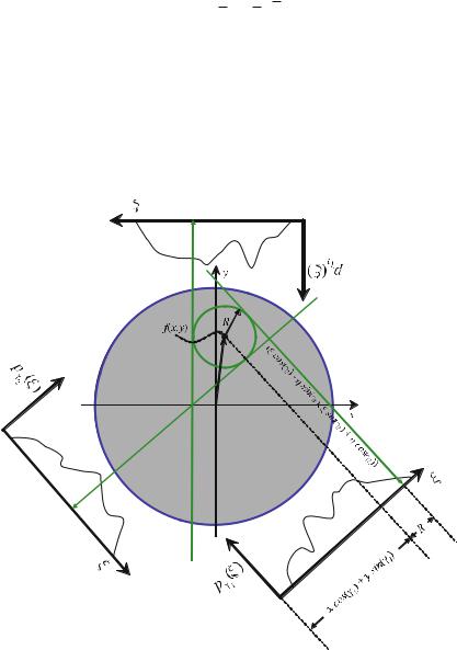

|
5 Two-Dimensional Fourier-Based Reconstruction Methods |
|
|
||||||||
|
which is along a straight line, can be written compactly as |
|
|||||||||
|
f δ |
L |
∫ f r δ |
rT |
ċ |
nξ |
) − |
ξ |
) |
dr |
( . ) |
|
using the sift property of>the( |
δ)-distribution.= ( ) (( |
|
|
|
|
|
||||
|
In fact, the projection values at the points |
|
|
|
|
|
|
|
|||
|
(x cos(γ) + y sin(γ) + R, γ) |
|
|
( . ) |
|||||||
in the Radon space are averaged. In order to reconstruct the image value f at the point (x, y)T the averaged values are weighted with the reciprocal value of the distance from that point and finally integrated. As this section started with ( . ), i.e., the filtered projection hγ (ξ), this point of view is obviously equivalent to the filtered backprojection.
The filtered backprojection can be written very compactly when using the definition of the Hilbert transform introduced in Sect. . .
With
|
& |
|
d( |
|
) |
' = |
|
− |
|
|
|
|
|
|
|
|
|
|
( |
|
) |
|
|
||
H |
|
dpγ |
ξ |
|
|
|
|
+ |
|
|
|
|
|
dpγ |
|
ξ |
|
dξ , |
( . ) |
||||||
|
|
ξ |
|
|
|
|
π |
∫ ξ |
− |
ξ |
|
|
|
|
dξ |
|
|
|
|||||||
|
|
|
|
|
|
|
|
|
|
|
|
|
|
|
|
||||||||||
( . ) can be written as |
|
|
( |
|
) = |
|
|
& |
d( |
|
)' |
|
|
|
|
|
|||||||||
|
|
|
|
|
|
|
|
|
ξ |
|
|
|
|
|
|||||||||||
|
|
|
hγ |
|
ξ |
|
|
|
H |
|
|
|
|
|
|
|
|
|
|
|
. |
|
|
|
( . ) |
|
|
|
|
|
|
|
|
π |
|
|
|
|
ξ |
|
|
|
|
|
|
|
|
|
|
||
This, along with ( . ) for the filtered backprojection, gives the expression |
|
||||||||||||||||||||||||
|
|
( |
|
) = |
|
|
π |
|
& d( )' |
|
|
|
|
|
|||||||||||
|
f |
|
x, y |
|
|
|
|
∫ H |
|
dpγ ξ |
|
|
|
|
dγ . |
( . ) |
|||||||||
|
|
|
|
|
π |
ξ |
|
|
|
|
|||||||||||||||
5.11
Cormack Transform
So far, only the vertical lines in the Cartesian Radon space have been considered, which, in terms of the measurement process, correspond to a complete projection signal acquired over an angle of . However, the previous section showing the relation between filtered backprojection and Radon’s original work, excerpts of which were translated at the beginning of Chap. , also suggests a di erent view on data in the Radon space.
In this section, data arranged on horizontal lines in the Radon space are considered. This perspective leads to a decomposition into what is called the circular
Strictly speaking, the derivation of p with respect to ξ is a partial derivative, so that ( . )
|
( |
|
) = |
|
π |
|
|
∂pγ (ξ) |
|
|
|
correctly reads f |
x, y |
∫ |
H |
|
dγ. |
||||||
|
|||||||||||
|
|
π |
|
∂ξ |
!ξ = x cos(γ)+ y sin(γ) |
||||||
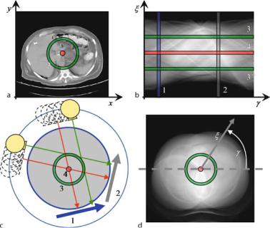
5.11 Cormack Transform |
|
harmonics. As this method was proposed by Cormack, it is frequently referred to it as the Cormack transform.
In Fig. . a once again an abdominal tomogram can be seen. The corresponding Cartesian Radon space reflecting the projection data from γ = to γ = is presented in Fig. . b. The horizontal lines in this diagram belong to certain circles in the spatial domain whose tangents are the corresponding projection lines. This is schematically illustrated in Fig. . c. In Fig. . d, the Radon space data are given in polar coordinates. Obviously, the horizontal lines in the Cartesian Radon space belong to certain circles in the polar diagram. The upper half ( − π) of the circle drawn on Fig. . a, c, and d corresponds to line drawn on Fig. . b, and the lower half of the circle (π − π) corresponds to line .
Due to the circular symmetry of the data acquisition system, every data ring pγ (ξ) = p(ξ, γ) is periodic in the projection angle γ , having period π. T hus, every ring can be written as a Fourier series
|
( |
|
) = |
|
|
( |
|
) |
|
|
p |
ξ, γ |
|
pn |
ξ |
einγ , |
( . ) |
||||
|
|
|
|
n =− |
|
|
|
|
|
|
Fig. . a–d. A decomposition into circular harmonics represents another view of Radon space data. Instead of the vertical lines and , one changes the perspective to the horizontal lines or and in the sinogram
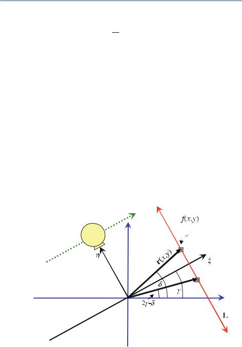

5.11 Cormack Transform
are determined separately, i.e.,
p(ξ, γ) = |
|
f (r, δ)dη + |
|
|
∫ |
∫ f (r, δ)dη . |
( . ) |
||
|
|
|
− |
|
Using the symmetry of Fig. . , the two integrals in ( . ) can be combined to give
p(ξ, γ) = |
|
f (r, δ) + f (r, γ − δ) dη . |
|
∫ |
( . ) |
Expressing the leftand right-hand sides of ( . ) by their Fourier expansions ( . ) and ( . ) respectively, one obtains
|
|
|
|
|
|
|
|
|
|
|
|
|
|
|
|
|
|
|
|
|
|
|
|
|
|
|
|
|
|
|
||
pn ξ einγ |
|
∫ |
|
|
|
fn r einδ |
|
|
|
fn r ein( γ−δ) dη |
|
|
|
|
|
|
||||||||||||||||
|
|
|
n =− |
|
|
|
|
|
|
|
|
|
|
|
||||||||||||||||||
n =− |
( ) = |
|
|
( ) + |
n =− |
( ) |
|
' |
|
|
|
|
|
|
|
|||||||||||||||||
|
|
|
& |
|
|
|
|
|
|
|
|
|
|
|
|
|
|
|||||||||||||||
|
|
|
|
|
∫ |
|
|
|
|
fn |
r |
|
|
einδ |
|
ein( γ−δ) |
' |
dη |
|
|
|
( . ) |
||||||||||
|
|
|
|
|
|
n =− |
|
|
|
|
|
|
||||||||||||||||||||
|
|
|
|
= |
|
|
( ) |
|
|
+ |
|
|
|
|
|
|
|
|
|
|
|
|
|
|
||||||||
|
|
|
|
|
& |
|
|
|
|
|
|
|
|
|
|
|
|
|
|
|
|
|
|
|||||||||
|
|
|
|
|
∫ |
|
|
|
|
fn r einγ ein(δ−γ) e−in(δ−γ) |
|
dη . |
|
|
|
|
|
|
||||||||||||||
|
|
|
|
|
|
n =− |
|
|
|
|
|
|
|
|||||||||||||||||||
|
|
|
|
= |
|
|
( ) |
|
|
|
|
|
|
|
|
+ |
|
|
' |
|
|
|
|
|
|
|
||||||
|
|
|
|
|
& |
|
|
|
|
|
|
|
|
|
|
|
|
|
|
|
|
|
|
|||||||||
Writing the cosine as its complex exponential functions |
|
|
|
|
|
|
|
|
|
|
||||||||||||||||||||||
( . ) can be simplified to |
|
|
cos(α) = |
eiα + e−iα |
|
, |
|
|
|
|
|
|
( . ) |
|||||||||||||||||||
|
|
|
|
|
|
|
|
|
|
|
|
|
|
|
|
|
|
|
|
|
|
|
|
|
|
|
|
|
|
|
|
|
|
pn ξ einγ |
|
∫ |
|
|
|
fn |
|
r einγ cos |
|
n δ |
γ |
dη . |
|
( . ) |
|||||||||||||||||
|
|
|
|
n |
=− |
|
|
|
||||||||||||||||||||||||
n =− |
( ) |
|
= |
|
|
|
& |
|
( ) |
|
|
|
|
( ( − |
))' |
|
|
|
|
|
|
|
|
|||||||||
|
|
|
|
|
|
|
|
|
|
|
|
|
|
|
|
|
|
|
|
|
|
|
||||||||||
Changing the coordinates |
( |
ξ, η |
) |
for the benefit of the polar presentation to |
( |
r, δ |
− |
γ |
) |
, |
||||||||||||||||||||||
where |
|
|
|
|
|
|
|
|
r = G |
|
|
|
|
|
|
|
|
|
|
|
|
|
|
|
||||||||
and |
|
|
|
|
|
|
|
|
|
|
ξ + η |
|
|
|
|
|
|
|
|
( . ) |
||||||||||||
|
|
|
|
|
|
|
|
|
|
ξ = r cos(δ − γ) , |
|
|
|
|
|
|
|
( . ) |
||||||||||||||
one can write the following after swapping the order of summation and integration
|
|
|
|
|
|
|
|
|
fn |
r |
|
cos |
|
n cos− |
|
ξ r |
|
|
|
||||||||||
n =− pn |
ξ |
) |
einγ |
= |
n =− einγ |
|
ξ∫ |
|
|
( |
) |
|
|
r |
− |
ξ |
( |
|
|
) |
r dr |
|
|||||||
|
( |
|
|
- |
|
|
|
|
|
|
|
|
G |
|
|
ξ r |
|
r drBeinγ . |
( . ) |
||||||||||
|
|
|
|
|
|
|
|
f |
n |
r |
|
cos n cos− |
|
|
|||||||||||||||
|
|
|
|
|
|
|
|
|
|
|
|
|
|
|
|
|
|
|
|
|
|
|
|
|
|||||
|
|
|
|
= |
n =− |
. |
ξ∫ |
|
|
|
( |
) |
|
|
r |
|
|
ξ |
|
|
( ) |
|
. |
|
|||||
|
|
|
|
|
/ |
|
|
|
|
|
|
|
|
G |
− |
|
|
|
|
|
|
|
|
C |
|
||||
|
|
|
|
|
|
. |
|
|
|
|
|
|
|
|
|
|
|
|
|
|
|
|
|
|
|
|
. |
|
|
|
|
|
|
|
|
0 |
|
|
|
|
|
|
|
|
|
|
|
|
|
|
|
|
|
|
|
|
|
D |
|

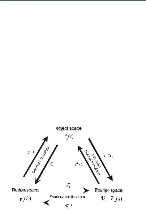

5 Two-Dimensional Fourier-Based Reconstruction Methods
These are written in a more compact way as |
|
|
and |
Pn(q) = in Hn fn (r) |
( . ) |
|
fn (r) = in Hn Pn (q) |
( . ) |
respectively. These are – as a generalization of the definition given in Sect. . – the Hankel transforms of the nth order. Figure . schematically represents the quantities discussed in this section. For rotationally symmetric objects, the Cormack transform can be identified with the Abel transformation of Sect. . .