


Thorsten M. Buzug
Computed Tomography

Thorsten M. Buzug
Computed Tomography
From Photon Statistics
to Modern Cone-Beam CT
With 475 Figures and 10 Tables
123

Thorsten M. Buzug, Prof. Dr.
Institut für Medizintechnik Universität zu Lübeck Ratzeburger AlleeLübeck
Germany
E-mail: buzug@imt.uni-luebeck.de
ISBN - - - - |
e-ISBN - - - - |
DOI . / - - - -
Library of Congress Control Number:
© Springer-Verlag Berlin Heidelberg
This work is subject to copyright. All rights are reserved, whether the whole or part of the material is concerned, specifically the rights of translation, reprinting, reuse of illustrations, recitation, broadcasting, reproduction on microfilm or in any other way, and storage in data banks. Duplication of this publication or parts thereof is permitted only under the provisions of the German Copyright Law of September , , in its current version, and permission for use must always be obtained from Springer. Violations are liable to prosecution under the German Copyright Law.
The use of designations, trademarks, etc. in this publication does not imply, even in the absence of a specific statement, that such names are exempt from the relevant protective laws and regulations and therefore free for general use.
Product liability: The publisher can not guarantee the accuracy of any information about dosage and application contained in this book. In every individual case the user must check such information by consulting the relevant literature.
Production and Typesetting: le-tex publishing services oHG, Leipzig, Germany Cover design: Frido Steinen-Broo, eStudio Calamar, Spain
Printed on acid-free paper
springer.com

Preface
This book provides an overview of X-ray technology, the historic developmental milestones of modern CT systems, and gives a comprehensive insight into the main reconstruction methods used in computed tomography. The basis of reconstruction is, undoubtedly, mathematics. However, the beauty of computed tomography cannot be understood without a detailed knowledge of X-ray generation, photon– matter interaction, X-ray detection, photon statistics, as well as fundamental signal processing concepts and dedicated measurement systems. Therefore, the reader will find a number of references to these basic disciplines together with a brief introduction to the underlying principles of CT.
This book is structured to cover the basics of CT: from photon statistics to modern cone-beam systems. However, the main focus of the book is concerned with detailed derivations of reconstruction algorithms in D and modern D cone-beam systems. A thorough analysis of CT artifacts and a discussion of practical issues, such as dose considerations, provide further insight into modern CT systems. While mainly written for graduate students in biomedical engineering, medical engineering science, medical physics, medicine (radiology), mathematics, electrical engineering, and physics, experienced practitioners in these fields will benefit from this book as well.
The didactic approach is based on consistent notation. For example, the notation of computed tomography is used in the signal processing chapter. Therefore, contrary to many other signal processing books, which use time-dependent values, this book uses spatial variables in one, two or three dimensions. This facilitates the application of the mathematics and physics learned from the earlier chapters to detector array signal processing, which is described in the later chapters. Additionally, special attention has been paid to creating a text with detailed and richly discussed algorithm derivations rather than compact mathematical presentations. The concepts should give even undergraduate students the chance to understand the principal reconstruction theory of computed tomography. The text is supported by a large number of illustrations representing the geometry of the projection situation. Since the impact of cone-beam CT will undeniably increase in the future, three-dimensional reconstruction algorithms are illustrated and derived in detail.
This book attempts to close a gap. There are several excellent books on medical imaging technology that give a comprehensive overview of modern X-ray technology, computed tomography, magnetic resonance imaging, ultrasound, or nuclear

VI Preface
medicine modalities like PET and SPECT. However, these books often do not go into the mathematical detail of signal processing theory. On the other hand, there are a number of in-depth mathematical books on computed tomography that do not discuss practical issues. The present book is based on the German book Einführung in die Computertomographie, which first appeared during the summer of. Fortunately, since the book was used by many of my students in lectures on
Engineering in Radiology, Medical Engineering, Signals and Systems in Medicine, and
Tomographic Methods, I received a lot of feedback regarding improvements on the first edition. Therefore, the idea arose to publish an English version of the book, which is a corrected and extended follow-up.
I would like to thank Siemens Medical Solutions, General Electric Medical Systems, and Philips Medical Systems, who generously supported my laboratories in the field of computed tomography. In particular, I would like to thank my friend Dr. Michael Kuhn, former Director of Philips Research Hamburg. It was his initiative that made possible the first installation of CT in my labs in . Additionally, I have to thank Mrs. Annette Halstrick and Dr. Hans-Dieter Nagel (Philips Medical Systems Hamburg), Leon de Vries (Philips Medical Systems Best), Doris Pischitz, Jürgen Greim and Robby Rokkitta (Siemens Medical Solutions Erlangen), Dieter Keidel and Jan Liedtke (General Electric Medical Systems) for many photos in this book. I would like to thank Wolfgang Härer (AXI CC, Siemens Medical Solutions), Dr. Gerhard Brunst, (General Electric Medical Systems), Dr. Armin H. Pfoh, Director of General Electric Research Munich, Dr. Wolfgang Niederlag (Hospital Dresden-Friedrichstadt), Prof. Dr. Heinz U. Lemke (Technical University Berlin), Dr. Henrik Turbell (Institute of Technology, Linköpings Universitet), and Prof. Dr. Dr. Jürgen Ruhlmann (Medical Center Bonn) for the courtesy to allow me to use their illustrations and photos. Further, I have to thank the Digital Collections and Archives of Tufts University, the Collection of Portraits of the Austrian Academy of Sciences, and the Röntgen-Kuratorium Würzburg e.V. for the courtesy to allow me to use their photos.
Additionally, I have to thank my friends, colleagues, and students for proofreading and translating parts of the book. In alphabetical order I appreciated the help of:
Dr. Bernd David (Philips Research Laboratories Hamburg) Katie Dechambre (Milwaukee School of Engineering)
Erin Fredericks (California Polytechnic State University, San Luis Obispo) Sebastian Gollmer (University of Lübeck)
Dr. Franko Greiner (University of Kiel)
Tobias Knopp (University of Lübeck) Dieter Lukhaup (Schriesheim-Altenbach) Andreas Mang (University of Lübeck)
Prof. Dr.-Ing. Alfred Mertins (University of Lübeck) Jan Müller (University of Lübeck)
Dr. Hans-Dieter Nagel (Philips Medical Systems Hamburg) Susanne Preissler (RheinAhrCampus Remagen)

Preface VII
Tony Shepherd (University College London)
Vyara Tonkova (RheinAhrCampus Remagen)
Many special thanks go to Sebastian Gollmer, Andreas Mang, and Jan Müller, who did the copy editing of the complete manuscript. However, for the errors that remain, I alone am responsible and apologize in advance.
I would like to thank the production team at le-tex as well as Paula Francis for copy editing. Further, I have to thank Springer Publishing, especially Dr. Ute Heilmann and Wilma McHugh for their excellent cooperation over the last few years.
Finally, I would like to thank my wife Kerstin, who has supported and sustained my writing e orts over the last few years. Without her help, patience, and encouragement this book would not have been completed.
Lübeck, June |
Thorsten M. Buzug |

Contents
1 |
Introduction |
. . . . . . . . . . . . . . . . . . . . . . . . . . . . . . . . . . . . . . . . . . . . . . . . . . . . . . . . |
1 |
|
|
. |
Computed Tomography – State of the Art . . . . . . . . . . . . . . . . . . . . . . . . . |
1 |
|
|
. |
Inverse Problems . . . . . . . . . . . . . . . . . . . . . . . . . . . . . . . . . . . . . . . . . . . . . . |
2 |
|
|
. |
Historical Perspective . . . . . . . . . . . . . . . . . . . . . . . . . . . . . . . . . . . . . . . . . . |
4 |
|
|
. |
Some Examples . . . . . . . . . . . . . . . . . . . . . . . . . . . . . . . . . . . . . . . . . . . . . . . . |
7 |
|
|
. |
Structure of the Book . . . . . . . . . . . . . . . . . . . . . . . . . . . . . . . . . . . . . . . . . . . |
11 |
|
2 |
Fundamentals of X-ray Physics . . . . . . . . . . . . . . . . . . . . . . . . . . . . . . . . . . . . . . . . |
15 |
||
|
. |
Introduction . . . . . . . . . . . . . . . . . . . . . . . . . . . . . . . . . . . . . . . . . . . . . . . . . . |
15 |
|
|
. |
X-ray Generation . . . . . . . . . . . . . . . . . . . . . . . . . . . . . . . . . . . . . . . . . . . . . . |
15 |
|
|
|
. . |
X-ray Cathode . . . . . . . . . . . . . . . . . . . . . . . . . . . . . . . . . . . . . . . . . . |
16 |
|
|
. . |
Electron–Matter Interaction . . . . . . . . . . . . . . . . . . . . . . . . . . . . . . |
19 |
|
|
. . |
Temperature Load . . . . . . . . . . . . . . . . . . . . . . . . . . . . . . . . . . . . . . . |
23 |
|
|
. . |
X-ray Focus and Beam Quality . . . . . . . . . . . . . . . . . . . . . . . . . . . . |
24 |
|
|
. . |
Beam Filtering . . . . . . . . . . . . . . . . . . . . . . . . . . . . . . . . . . . . . . . . . . |
28 |
|
|
. . |
Special Tube Designs . . . . . . . . . . . . . . . . . . . . . . . . . . . . . . . . . . . . |
30 |
|
. |
Photon–Matter Interaction . . . . . . . . . . . . . . . . . . . . . . . . . . . . . . . . . . . . . . |
31 |
|
|
|
. . |
Lambert–Beer’s Law . . . . . . . . . . . . . . . . . . . . . . . . . . . . . . . . . . . . . |
32 |
|
|
. . |
Mechanisms of Attenuation . . . . . . . . . . . . . . . . . . . . . . . . . . . . . . |
34 |
|
. |
Problems with Lambert–Beer’s Law . . . . . . . . . . . . . . . . . . . . . . . . . . . . . . |
46 |
|
|
. |
X-ray Detection . . . . . . . . . . . . . . . . . . . . . . . . . . . . . . . . . . . . . . . . . . . . . . . |
48 |
|
|
|
. . |
Gas Detectors . . . . . . . . . . . . . . . . . . . . . . . . . . . . . . . . . . . . . . . . . . . |
48 |
|
|
. . |
Solid-State Scintillator Detectors . . . . . . . . . . . . . . . . . . . . . . . . . . |
50 |
|
|
. . |
Solid-State Flat-Panel Detectors . . . . . . . . . . . . . . . . . . . . . . . . . . . |
52 |
|
. |
X-ray Photon Statistics . . . . . . . . . . . . . . . . . . . . . . . . . . . . . . . . . . . . . . . . . |
59 |
|
|
|
. . |
Statistical Properties of the X-ray Source . . . . . . . . . . . . . . . . . . . |
60 |
|
|
. . |
Statistical Properties of the X-ray Detector . . . . . . . . . . . . . . . . . |
64 |
|
|
. . |
Statistical Law of Attenuation . . . . . . . . . . . . . . . . . . . . . . . . . . . . . |
66 |
|
|
. . |
Moments of the Poisson Distribution . . . . . . . . . . . . . . . . . . . . . . |
68 |
|
|
. . |
Distribution for a High Number of X-ray Quanta . . . . . . . . . . . |
70 |
|
|
. . |
Non-Poisson Statistics . . . . . . . . . . . . . . . . . . . . . . . . . . . . . . . . . . . |
72 |

XContents
3 |
Milestones of Computed Tomography . . . . . . . . . . . . . . . . . . . . . . . . . . . . . . . . . |
75 |
||
|
. |
Introduction . . . . . . . . . . . . . . . . . . . . . . . . . . . . . . . . . . . . . . . . . . . . . . . . . . |
75 |
|
|
. |
Tomosynthesis . . . . . . . . . . . . . . . . . . . . . . . . . . . . . . . . . . . . . . . . . . . . . . . . |
76 |
|
|
. |
Rotation–Translation of a Pencil Beam (First Generation) . . . . . . . . . . . |
79 |
|
|
. |
Rotation–Translation of a Narrow Fan Beam (Second Generation) . . . |
83 |
|
|
. |
Rotation of a Wide Aperture Fan Beam (Third Generation) . . . . . . . . . |
84 |
|
|
. |
Rotation–Fix with Closed Detector Ring (Fourth Generation) . . . . . . . |
87 |
|
|
. |
Electron Beam Computerized Tomography . . . . . . . . . . . . . . . . . . . . . . . |
89 |
|
|
. |
Rotation in Spiral Path. . . . . . . . . . . . . . . . . . . . . . . . . . . . . . . . . . . . . . . . . . |
90 |
|
|
. |
Rotation in Cone-Beam Geometry . . . . . . . . . . . . . . . . . . . . . . . . . . . . . . . |
91 |
|
|
. |
Micro-CT . . . . . . . . . . . . . . . . . . . . . . . . . . . . . . . . . . . . . . . . . . . . . . . . . . . . . |
93 |
|
|
. |
PET-CT Combined Scanners . . . . . . . . . . . . . . . . . . . . . . . . . . . . . . . . . . . . |
96 |
|
|
. |
Optical Reconstruction Techniques . . . . . . . . . . . . . . . . . . . . . . . . . . . . . . |
98 |
|
4 |
Fundamentals of Signal Processing . . . . . . . . . . . . . . . . . . . . . . . . . . . . . . . . . . . . |
101 |
||
|
. |
Introduction . . . . . . . . . . . . . . . . . . . . . . . . . . . . . . . . . . . . . . . . . . . . . . . . . . |
102 |
|
|
. |
Signals |
. . . . . . . . . . . . . . . . . . . . . . . . . . . . . . . . . . . . . . . . . . . . . . . . . . . . . . . . |
102 |
|
. |
Fundamental Signals . . . . . . . . . . . . . . . . . . . . . . . . . . . . . . . . . . . . . . . . . . . |
102 |
|
|
. |
Systems . . . . . . . . . . . . . . . . . . . . . . . . . . . . . . . . . . . . . . . . . . . . . . . . . . . . . . . |
104 |
|
|
|
. . |
Linearity . . . . . . . . . . . . . . . . . . . . . . . . . . . . . . . . . . . . . . . . . . . . . . . |
104 |
|
|
. . |
Position or Translation Invariance . . . . . . . . . . . . . . . . . . . . . . . . . |
105 |
|
|
. . |
Isotropy and Rotation Invariance . . . . . . . . . . . . . . . . . . . . . . . . . . |
105 |
|
|
. . Causality . . . . . . . . . . . . . . . . . . . . . . . . . . . . . . . . . . . . . . . . . . . . . . . |
106 |
|
|
|
. . Stability . . . . . . . . . . . . . . . . . . . . . . . . . . . . . . . . . . . . . . . . . . . . . . . . |
106 |
|
|
. |
Signal Transmission . . . . . . . . . . . . . . . . . . . . . . . . . . . . . . . . . . . . . . . . . . . . |
106 |
|
|
. |
Dirac’s Delta Distribution . . . . . . . . . . . . . . . . . . . . . . . . . . . . . . . . . . . . . . . |
109 |
|
|
. |
Dirac Comb . . . . . . . . . . . . . . . . . . . . . . . . . . . . . . . . . . . . . . . . . . . . . . . . . . . |
112 |
|
|
. |
Impulse Response . . . . . . . . . . . . . . . . . . . . . . . . . . . . . . . . . . . . . . . . . . . . . . |
115 |
|
|
. |
Transfer Function . . . . . . . . . . . . . . . . . . . . . . . . . . . . . . . . . . . . . . . . . . . . . . |
116 |
|
|
. |
Fourier Transform . . . . . . . . . . . . . . . . . . . . . . . . . . . . . . . . . . . . . . . . . . . . . |
118 |
|
|
. |
Convolution Theorem . . . . . . . . . . . . . . . . . . . . . . . . . . . . . . . . . . . . . . . . . . |
124 |
|
|
. |
Rayleigh’s Theorem . . . . . . . . . . . . . . . . . . . . . . . . . . . . . . . . . . . . . . . . . . . . . |
125 |
|
|
. |
Power Theorem . . . . . . . . . . . . . . . . . . . . . . . . . . . . . . . . . . . . . . . . . . . . . . . . |
125 |
|
|
. |
Filtering in the Frequency Domain . . . . . . . . . . . . . . . . . . . . . . . . . . . . . . . |
126 |
|
|
. |
Hankel Transform . . . . . . . . . . . . . . . . . . . . . . . . . . . . . . . . . . . . . . . . . . . . . |
128 |
|
|
. |
Abel Transform . . . . . . . . . . . . . . . . . . . . . . . . . . . . . . . . . . . . . . . . . . . . . . . . |
132 |
|
|
. |
Hilbert Transform . . . . . . . . . . . . . . . . . . . . . . . . . . . . . . . . . . . . . . . . . . . . . |
133 |
|
|
. |
Sampling Theorem and Nyquist Criterion . . . . . . . . . . . . . . . . . . . . . . . . . |
135 |
|
|
. |
Wiener–Khintchine Theorem. . . . . . . . . . . . . . . . . . . . . . . . . . . . . . . . . . . . |
141 |
|
|
. |
Fourier Transform of Discrete Signals . . . . . . . . . . . . . . . . . . . . . . . . . . . . |
144 |
|
|
. |
Finite Discrete Fourier Transform . . . . . . . . . . . . . . . . . . . . . . . . . . . . . . . . |
145 |
|
|
. |
z-Transform . . . . . . . . . . . . . . . . . . . . . . . . . . . . . . . . . . . . . . . . . . . . . . . . . . . |
147 |
|
|
. |
Chirp z-Transform . . . . . . . . . . . . . . . . . . . . . . . . . . . . . . . . . . . . . . . . . . . . . |
148 |
|

Contents XI
5 Two-Dimensional Fourier-Based Reconstruction Methods . . . . . . . . . . . . . . . 151
. Introduction . . . . . . . . . . . . . . . . . . . . . . . . . . . . . . . . . . . . . . . . . . . . . . . . . . 151
. Radon Transformation . . . . . . . . . . . . . . . . . . . . . . . . . . . . . . . . . . . . . . . . . 153
. Inverse Radon Transformation and Fourier Slice Theorem . . . . . . . . . . 163
. Implementation of the Direct Inverse Radon Transform . . . . . . . . . . . . 167
. Linogram Method . . . . . . . . . . . . . . . . . . . . . . . . . . . . . . . . . . . . . . . . . . . . . 170
. Simple Backprojection . . . . . . . . . . . . . . . . . . . . . . . . . . . . . . . . . . . . . . . . . . 175
. Filtered Backprojection . . . . . . . . . . . . . . . . . . . . . . . . . . . . . . . . . . . . . . . . . 179
. Comparison Between Backprojection and Filtered Backprojection . . . 183
. Filtered Layergram: Deconvolution of the Simple Backprojection . . . . 187
. Filtered Backprojection and Radon’s Solution . . . . . . . . . . . . . . . . . . . . . . 191
. Cormack Transform . . . . . . . . . . . . . . . . . . . . . . . . . . . . . . . . . . . . . . . . . . . . 194
6 Algebraic and Statistical Reconstruction Methods . . . . . . . . . . . . . . . . . . . . . . . 201
. Introduction . . . . . . . . . . . . . . . . . . . . . . . . . . . . . . . . . . . . . . . . . . . . . . . . . . 201
. Solution with Singular Value Decomposition . . . . . . . . . . . . . . . . . . . . . . 207
. Iterative Reconstruction with ART . . . . . . . . . . . . . . . . . . . . . . . . . . . . . . . 211
. Pixel Basis Functions and Calculation of the System Matrix . . . . . . . . . 218. . Discretization of the Image: Pixels and Blobs . . . . . . . . . . . . . . . 219. . Approximation of the System Matrix in the Case of Pixels . . . . 221. . Approximation of the System Matrix in the Case of Blobs . . . . 222
. Maximum Likelihood Method . . . . . . . . . . . . . . . . . . . . . . . . . . . . . . . . . . . 223
. . Maximum Likelihood Method for Emission Tomography . . . . 224. . Maximum Likelihood Method for Transmission CT . . . . . . . . . 230. . Regularization of the Inverse Problem . . . . . . . . . . . . . . . . . . . . . 235. . Approximation Through Weighted Least Squares . . . . . . . . . . . . 238
7 Technical Implementation . . . . . . . . . . . . . . . . . . . . . . . . . . . . . . . . . . . . . . . . . . . . 241. Introduction . . . . . . . . . . . . . . . . . . . . . . . . . . . . . . . . . . . . . . . . . . . . . . . . . . 241. Reconstruction with Real Signals . . . . . . . . . . . . . . . . . . . . . . . . . . . . . . . . 242. . Frequency Domain Windowing . . . . . . . . . . . . . . . . . . . . . . . . . . . 244
. . Convolution in the Spatial Domain . . . . . . . . . . . . . . . . . . . . . . . . 247
. . Discretization of the Kernels . . . . . . . . . . . . . . . . . . . . . . . . . . . . . . 252
. Practical Implementation of the Filtered Backprojection . . . . . . . . . . . . 255. . Filtering of the Projection Signal . . . . . . . . . . . . . . . . . . . . . . . . . . 255. . Implementation of the Backprojection . . . . . . . . . . . . . . . . . . . . . 258
. Minimum Number of Detector Elements . . . . . . . . . . . . . . . . . . . . . . . . . 258
. Minimum Number of Projections . . . . . . . . . . . . . . . . . . . . . . . . . . . . . . . . 259. Geometry of the Fan-Beam System . . . . . . . . . . . . . . . . . . . . . . . . . . . . . . . 261
. Image Reconstruction for Fan-Beam Geometry . . . . . . . . . . . . . . . . . . . . 262
. . Rebinning of the Fan Beams . . . . . . . . . . . . . . . . . . . . . . . . . . . . . . 265. . Complementary Rebinning . . . . . . . . . . . . . . . . . . . . . . . . . . . . . . . 270
XII |
Contents |
|
|
|
|
|
|
|
. . |
Filtered Backprojection for Curved Detector Arrays . . . . . . . . . |
272 |
|
|
|
. . |
Filtered Backprojection for Linear Detector Arrays . . . . . . . . . . |
280 |
|
|
|
. . |
Discretization of Backprojection for Fan-Beam Geometry . . . . |
286 |
|
|
. |
Quarter-Detector O set and Sampling Theorem . . . . . . . . . . . . . . . . . . . |
293 |
|
|
8 |
Three-Dimensional Fourier-Based Reconstruction Methods . . . . . . . . . . . . . . |
303 |
||
|
|
. |
Introduction . . . . . . . . . . . . . . . . . . . . . . . . . . . . . . . . . . . . . . . . . . . . . . . . . . |
303 |
|
|
|
. |
Secondary Reconstruction Based on 2D Stacks of Tomographic Slices |
304 |
|
|
|
. |
Spiral CT . . . . . . . . . . . . . . . . . . . . . . . . . . . . . . . . . . . . . . . . . . . . . . . . . . . . . |
309 |
|
|
|
. |
Exact 3D Reconstruction in Parallel-Beam Geometry . . . . . . . . . . . . . . |
321 |
|
|
|
|
. . |
3D Radon Transform and the Fourier Slice Theorem . . . . . . . . . |
321 |
|
|
|
. . |
Three-Dimensional Filtered Backprojection . . . . . . . . . . . . . . . . |
326 |
|
|
|
. . |
Filtered Backprojection and Radon’s Solution . . . . . . . . . . . . . . . |
327 |
|
|
|
. . |
Central Section Theorem . . . . . . . . . . . . . . . . . . . . . . . . . . . . . . . . . |
329 |
|
|
|
. . |
Orlov’s Su ciency Condition . . . . . . . . . . . . . . . . . . . . . . . . . . . . . |
335 |
|
|
. |
Exact 3D Reconstruction in Cone-Beam Geometry . . . . . . . . . . . . . . . . |
336 |
|
|
|
|
. . |
Key Problem of Cone-Beam Geometry . . . . . . . . . . . . . . . . . . . . |
339 |
|
|
|
. . |
Method of Grangeat . . . . . . . . . . . . . . . . . . . . . . . . . . . . . . . . . . . . . |
341 |
|
|
|
. . |
Computation of the First Derivative on the Detector . . . . . . . . . |
347 |
|
|
|
. . |
Reconstruction with the Derivative of the Radon Transform . . |
348 |
|
|
|
. . |
Central Section Theorem and Grangeat’s Solution . . . . . . . . . . . |
350 |
|
|
|
. . |
Direct 3D Fourier Reconstruction with the Cone-Beam |
354 |
|
|
|
|
Geometry . . . . . . . . . . . . . . . . . . . . . . . . . . . . . . . . . . . . . . . . . . . . . . |
|
|
|
|
. . |
Exact Reconstruction using Filtered Backprojection . . . . . . . . . |
357 |
|
|
. |
Approximate 3D Reconstructions in Cone-Beam Geometry . . . . . . . . . |
366 |
|
|
|
|
. . |
Missing Data in the 3D Radon Space . . . . . . . . . . . . . . . . . . . . . . |
366 |
|
|
|
. . |
FDK Cone-Beam Reconstruction for Planar Detectors . . . . . . . |
371 |
|
|
|
. . |
FDK Cone-Beam Reconstruction for Cylindrical Detectors . . . |
388 |
|
|
|
. . |
Variations of the FDK Cone-Beam Reconstruction . . . . . . . . . . |
390 |
|
|
. |
Helical Cone-Beam Reconstruction Methods . . . . . . . . . . . . . . . . . . . . . . |
394 |
|
|
9 |
Image Quality and Artifacts . . . . . . . . . . . . . . . . . . . . . . . . . . . . . . . . . . . . . . . . . . |
403 |
||
|
|
. |
Introduction . . . . . . . . . . . . . . . . . . . . . . . . . . . . . . . . . . . . . . . . . . . . . . . . . . |
403 |
|
|
|
. |
Modulation Transfer Function of the Imaging Process . . . . . . . . . . . . . . |
404 |
|
|
|
. |
Modulation Transfer Function and Point Spread Function . . . . . . . . . . |
410 |
|
|
|
. |
Modulation Transfer Function in Computed Tomography . . . . . . . . . . |
412 |
|
|
|
. |
SNR, DQE, and ROC . . . . . . . . . . . . . . . . . . . . . . . . . . . . . . . . . . . . . . . . . . . |
421 |
|
|
|
. |
2D Artifacts . . . . . . . . . . . . . . . . . . . . . . . . . . . . . . . . . . . . . . . . . . . . . . . . . . . |
423 |
|
|
|
|
. . |
Partial Volume Artifacts . . . . . . . . . . . . . . . . . . . . . . . . . . . . . . . . . |
423 |
|
|
|
. . |
Beam-Hardening Artifacts . . . . . . . . . . . . . . . . . . . . . . . . . . . . . . . |
425 |
|
|
|
. . |
Motion Artifacts . . . . . . . . . . . . . . . . . . . . . . . . . . . . . . . . . . . . . . . . |
432 |
|
|
|
. . |
Sampling Artifacts . . . . . . . . . . . . . . . . . . . . . . . . . . . . . . . . . . . . . . |
435 |
|
|
|
. . |
Electronic Artifacts . . . . . . . . . . . . . . . . . . . . . . . . . . . . . . . . . . . . . . |
435 |
|
|
|
. . |
Detector Afterglow . . . . . . . . . . . . . . . . . . . . . . . . . . . . . . . . . . . . . . |
437 |
|
|
|
. . |
Metal Artifacts . . . . . . . . . . . . . . . . . . . . . . . . . . . . . . . . . . . . . . . . . . |
438 |

Contents XIII
. . Scattered Radiation Artifacts . . . . . . . . . . . . . . . . . . . . . . . . . . . . . 443. 3D Artifacts . . . . . . . . . . . . . . . . . . . . . . . . . . . . . . . . . . . . . . . . . . . . . . . . . . . 445. . Partial Volume Artifacts . . . . . . . . . . . . . . . . . . . . . . . . . . . . . . . . . 446. . Staircasing in Slice Stacks . . . . . . . . . . . . . . . . . . . . . . . . . . . . . . . . 448. . Motion Artifacts . . . . . . . . . . . . . . . . . . . . . . . . . . . . . . . . . . . . . . . . 450
. . Shearing in Slice Stacks Due to Gantry Tilt . . . . . . . . . . . . . . . . . 451. . Sampling Artifacts in Secondary Reconstruction . . . . . . . . . . . . 454
. . Metal Artifacts in Slice Stacks . . . . . . . . . . . . . . . . . . . . . . . . . . . . . 455. . Spiral CT Artifacts . . . . . . . . . . . . . . . . . . . . . . . . . . . . . . . . . . . . . . 456. . Cone-Beam Artifacts . . . . . . . . . . . . . . . . . . . . . . . . . . . . . . . . . . . . 458
. . Segmentation and Triangulation Inaccuracies . . . . . . . . . . . . . . . 459
. Noise in Reconstructed Images . . . . . . . . . . . . . . . . . . . . . . . . . . . . . . . . . . 462
. . Variance of the Radon Transform . . . . . . . . . . . . . . . . . . . . . . . . . 462. . Variance of the Reconstruction . . . . . . . . . . . . . . . . . . . . . . . . . . . 464
. . Dose, Contrast, and Variance . . . . . . . . . . . . . . . . . . . . . . . . . . . . . 467
10 Practical Aspects of Computed Tomography . . . . . . . . . . . . . . . . . . . . . . . . . . . . 471
. Introduction . . . . . . . . . . . . . . . . . . . . . . . . . . . . . . . . . . . . . . . . . . . . . . . . . . 471. Scan Planning . . . . . . . . . . . . . . . . . . . . . . . . . . . . . . . . . . . . . . . . . . . . . . . . . 471. Data Representation . . . . . . . . . . . . . . . . . . . . . . . . . . . . . . . . . . . . . . . . . . . . 475. . Hounsfield Units . . . . . . . . . . . . . . . . . . . . . . . . . . . . . . . . . . . . . . . . 475
. . Window Width and Window Level . . . . . . . . . . . . . . . . . . . . . . . . 476. . Three-Dimensional Representation . . . . . . . . . . . . . . . . . . . . . . . 479
. Some Applications in Medicine . . . . . . . . . . . . . . . . . . . . . . . . . . . . . . . . . . 482
11 Dose . . . . . . . . . . . . . . . . . . . . . . . . . . . . . . . . . . . . . . . . . . . . . . . . . . . . . . . . . . . . . . . 485. Introduction . . . . . . . . . . . . . . . . . . . . . . . . . . . . . . . . . . . . . . . . . . . . . . . . . . 485
. Energy Dose, Equivalent Dose, and E ective Dose . . . . . . . . . . . . . . . . . 486. Definition of Specific CT Dose Measures . . . . . . . . . . . . . . . . . . . . . . . . . . 487. Device-Related Measures for Dose Reduction . . . . . . . . . . . . . . . . . . . . . 493. User-Related Measures for Dose Reduction . . . . . . . . . . . . . . . . . . . . . . . 499
References . . . . . . . . . . . . . . . . . . . . . . . . . . . . . . . . . . . . . . . . . . . . . . . . . . . . . . . . . 503
Subject Index . . . . . . . . . . . . . . . . . . . . . . . . . . . . . . . . . . . . . . . . . . . . . . . . . . . . . . |
511 |

1Introduction
Contents |
|
|
1.1 |
Computed Tomography – State of the Art . . . . . . . . . . . . . . . . . . . . . . . . . . . . . . . . . . |
1 |
1.2 |
Inverse Problems . . . . . . . . . . . . . . . . . . . . . . . . . . . . . . . . . . . . . . . . . . . . . . . . . . . . |
2 |
1.3 |
Historical Perspective . . . . . . . . . . . . . . . . . . . . . . . . . . . . . . . . . . . . . . . . . . . . . . . . . |
4 |
1.4 |
Some Examples . . . . . . . . . . . . . . . . . . . . . . . . . . . . . . . . . . . . . . . . . . . . . . . . . . . . . |
7 |
1.5 |
Structure of the Book . . . . . . . . . . . . . . . . . . . . . . . . . . . . . . . . . . . . . . . . . . . . . . . . . |
11 |
1.1
Computed Tomography – State of the Art
Computed tomography (CT) has evolved into an indispensable imaging method in clinical routine. It was the first method to non-invasively acquire images of the inside of the human body that were not biased by superposition of distinct anatomical structures. This is due to the projection of all the information into a twodimensional imaging plane, as typically seen in planar X-ray fluoroscopy. Therefore, CT yields images of much higher contrast compared with conventional radiography. During the s, this was an enormous step toward the advance of diagnostic possibilities in medicine.
However, research in the field of CT is still as exciting as at the beginning of its development during the s and s; however, several competing methods exist, the most important being magnetic resonance imaging (MRI). Since the invention of MRI during the s, the phasing out of CT has been anticipated. Nevertheless, to date, the most widely used imaging technology in radiology departments is still CT. Although MRI and positron emission tomography (PET) have been widely installed in radiology and in nuclear medicine departments, the term tomography is clearly associated with X-ray computed tomography .
Some hospitals actually replace their conventional shock rooms with a CTbased virtual shock room. In this scenario, imaging and primary care of the patient takes place using a CT scanner equipped with anesthesia devices. In a situation
In the United States computed tomography is also called CAT (computerized axial tomography).

1 Introduction
where the fast three-dimensional imaging of a trauma patient is necessary (and it is unclear whether MRI is an adequate imaging method in terms of compatibility with this patient), computed tomography is the standard imaging modality. Additionally, due to its ease of use, clear interpretation in terms of physical attenuation values, progress in detector technology, reconstruction mathematics, and reduction of radiation exposure, computed tomography will maintain and expand its established position in the field of radiology.
Furthermore, the preoperatively acquired CT image stack can be used to synthetically compute projections for any given angulations. A surgeon can use this information in order to get an impression of the images that are taken intraoperatively by a C-arm image intensifier. Therefore, there is no need to acquire additional radiographs and the artificially generated projection images actually resemble conventional radiographs. Additionally, the German Employer’s Liability Insurance Association insists on a CT examination in severe accidents that occur at work. Therefore, CT has advanced to become the standard diagnostic imaging modality in trauma clinics. Patients with heavy trauma, fractures, and luxations benefit greatly from the clarification provided by imaging techniques such as computed tomography.
Recently, interesting technical, anthropomorphic, forensic, and archeological (Thomsen et al. ) as well as paleontological (Pol et al. ) applications of computed tomography have been developed. These applications further strengthen the method as a generic diagnostic tool for non-destructive material testing and three-dimensional visualization beyond its medical use. Magnetic resonance imaging fails whenever the object to be examined is dehydrated. In these circumstances, computed tomography is the three-dimensional imaging method of choice.
1.2
Inverse Problems
The mathematics of CT image reconstruction has influenced other scientific fields and vice versa. The backprojection technique, for instance, is used in both geophysics and radar applications (Nilsson ). Clearly, the fundamental problem of computed tomography can be easily described: Reconstruct an object from its shadows or, more precisely, from its projections. An X-ray source with a fanor cone-beam geometry penetrates the object to be examined as a patient in medical applications, a skull found in archeology or a specimen in nondestructive testing (NDT). In the so-called third generation scanners, the fan-shaped X-ray beam fully covers a slice section of the object to be examined.
Depending on the particular paths, the X-rays are attenuated at varying extents when running through the object; the local absorption is measured with a detector array. Of course, the shadow that is cast in only one direction is not an adequate basis for the determination of the spatial distribution of distinct structures inside a three-dimensional object. In order to determine this structure, it is necessary to

1.2 Inverse Problems |
|
irradiate the object from all directions. Figure . schematically illustrates this principle, where pγi (ξ) represents the attenuation profile of the beam versus the X-ray detector array coordinate ξ under a particular projection angle γi . If the di erent attenuation or absorption profiles are plotted over all angles of rotation γi of the sampling unit, a sinusoidal arrangement of the attenuation or projection integral values is obtained. In two dimensions, these data, pγi (ξ), represent the radon space of the object, which is essentially the set of raw data.
In a special CT acquisition protocol, the spiral measurement process, the X-ray tube is continuously rotated, with the examination table being moved linearly through the measuring field. This scan process produces data that take a spiral or helical path. This method o ers the possibility of computing any number of slices retrospectively, so that an accurate three-dimensional rendering can be expected. To allow this acquisition technique, a slip ring transfer system has been developed. In such a system, power supply to the X-ray tube and signal transfer from the detector system is guaranteed, even though the imaging system continuously rotates.
From a mathematical point of view, image reconstruction in computed tomography is the task of computing the spatial structure of an object that casts shadows using these very shadows. The solution for this problem is complex and involves techniques in physics, mathematics, and computer science. The described scenario is referred to as the inverse problem in mathematics.
Fig. . . Schematic illustration of computed tomography (CT). Three homogeneous objects with quadratic intersection areas are exposed with X-ray under the projection angles γ and γ . Each projection angle produces a specific shadow, pγ (ξ), which, measured with the detector array represents the integral X-ray attenuation profile. The geometric shadow boundaries are indicated with dashed lines. However, analysis of the profile under the first projection angle, γ , on its own does not allow one to deduce an estimate of the number of separated objects

1 Introduction
1.3
Historical Perspective
A particular kind of mathematical problem in CT became popular in the s when the astrophysicist Bracewell proved that the resolution of telescopes could be significantly improved if spatially distributed telescopes are appropriately synchronized. However, in , similar problems with the same mathematical basis had already been discussed (cf. Cormack [ ] and the references therein; many examples are collected by Deans [ ]).
One example can be found in the field of statistics: Given all marginal distributions of a probability distribution density, is it possible to deduce the probability density itself? In this example, the marginal distributions represent an equivalent example for the measured projections in computed tomography. Another example can be found in astrophysics: Looking from earth into a particular direction of the universe, only the radial velocity component of the stars can be obtained via the spectral Doppler red shift. This again represents the same inverse problem that has to be solved if the distribution of the actual three-dimensional velocity vector is to be reconstructed from the radial velocity components acquired from all available directions.
In computed tomography, the meaning of the mathematical term inverse problem is immediately apparent. In contrast to the situation shown in Fig. . , the spatial distribution of the attenuating objects that produce the projection shadow is not known a priori. This, actually, is the reason for acquiring the projections along the rotating detector coordinate ξ over a projection angle interval of at least . Figure . illustrates this situation. It is an inversion of integral transforms. From a sequence of measured projection shadows pγ (ξ), pγ (ξ), pγ (ξ), . . . , the spa-
Fig. . . Schematic illustration of the inverse problem posed by CT. Attenuation profiles, pγ (ξ), have been measured for a set of projection angulations, γ and γ . The unknown geometry, or the object with its associated spatial distribution of attenuation coe cients, has to be calculated from a complete set of attenuation profiles pγ (ξ), pγ (ξ), pγ (ξ), . . .
1.3 Historical Perspective |
|
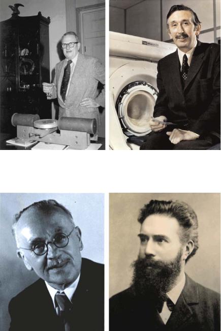
Fig. . . Left: Allan MacLeod Cormack ( – ) shortly after the o cial announcement of the Nobel Prizes for medicine in (courtesy of Tufts University, Digital Collections and Archives). Right: Sir Godfrey Hounsfield ( – ) in front of his first EMI CT scanner (courtesy of General Electric Medical Systems)
Fig. . . Left: Johann Radon ( – ; courtesy of the Austrian Academy of Sciences [OAW], collection of portraits). Right: Wilhelm Conrad Röntgen ( – ; courtesy of Röntgen-Kuratorium Würzburg e.V.)

1 Introduction
tial distribution of the objects, or more precisely, the spatial distribution of the attenuation coe cients within a chosen section through the patient, must be estimated.
In , the solution to this problem was applied for the first time to a sequence of X-ray projections for which an anatomical object had been measured from di erent directions. Allen MacLeod Cormack ( – ) and Sir Godfrey Hounsfield ( – ) are pioneers of medical computed tomography and in received the Nobel Prize for Medicine for their epochal work during the s and s. Figure . shows a picture of the two Nobel Prize winners.
Table . . Summary of historical CT milestones
Year Milestone
Röntgen discovers a new kind of radiation, which he named X-ray
Röntgen receives the Nobel Prize for physics
Bockwinkel employs the Lorentz’s solution in the reconstruction of threedimensional functions from two-dimensional area integrals
Radon publishes his epochal work on the solution of the inverse problem of reconstruction
Ehrenfest extends the solution of Lorentz to n dimensions using the Fourier transform
Cramer and Wold solve the reconstruction problem in statistics in which the probability distribution is obtained from a complete set of marginal probability distributions
Eddington solves the reconstruction problem in the field of astrophysics to calculate the distribution of star velocities from the distribution of their measured radial components
Bracewell applies Fourier techniques for the solution of the inverse problem in radio astronomy
The Ukrainian scientist Korenblyum develops an X-ray scanner and tries to measure thin slices through the patient with analogue reconstruction principles
Cormack contributes the first mathematical implementations for tomographic reconstruction in South Africa
Hounsfield shows proof of the principle with the first CT scanner based on a radioactive source at the EMI research laboratories
Hounsfield and Ambrose publish the first clinical scans with an EMI head scanner
Set-up of the first whole body scanner with a fan-beam system
Hounsfield and Cormack receive the Nobel Prize for Medicine
Demonstration of electron beam CT (EBCT)
Kalender publishes the first clinical spiral-CT
Demonstration of multi-slice CT (MSCT)
1.4 Some Examples |
|
Cormack pointed out that previously the Dutch physicist H.A. Lorentz had found a solution to the three-dimensional problem in which the desired function had to be reconstructed from two-dimensional surface integrals (Cormack ). Lorentz himself did not publish the results and so, unfortunately, the context of his work is still unknown today. The result, however, is associated with Lorentz by H. Bockwinkel, who mentioned the work in a publication on light propagation in crystals.
A detailed, mathematical basis to the solution of the inverse problem in computed tomography was published by the Bohemian mathematician Johann Radon in (cf. Fig. . , left) (Radon ). Due to the complexity and depth of the mathematical publication, however, the consequences of his ground-breaking results were revealed very late in the midth century. Additionally, the paper was published in German, which hindered a wide distribution of the work. In Chap. , an excerpt of his original work is reprinted.
In Table . , some of the historical milestones and development steps of computed tomography are summarized. The list undoubtedly has to start with Wilhelm Conrad Röntgen ( – ), who received the Nobel Prize for physics in (cf. Fig. . , right). Before , a significant number of mathematical contributions in the field of inverse problems were developed independently and are summarized here only retrospectively.
1.4
Some Examples
Figures . to . show several examples of computer tomographic images that illustrate di erent anatomical regions often used in clinical practice. Modern CT scanners yield images with an excellent soft tissue contrast. In Fig. . , the slices are annotated with the relevant scan protocol parameter. The most important parameters are the acceleration voltage (which determines the energy of the X-ray quanta), the tube current (which determines the intensity of the radiation), the slice thickness (which is the axial thickness of the X-ray fan beam), and the gantry tilt (which is the angulation of the CT frame with respect to the axial axis). In spiral-CT, the pitch is an additional parameter that defines the table feed in units of slice thickness.
In clinical practice, besides choosing an appropriate set of scan parameters (cf. Figs. . and . ), it is necessary to have a planning step for accurate anatomical scanning before CT slice sequence acquisition. In this planning step, the slices must be adapted to the anatomical situation, and furthermore, the dose for sensitive organs must be minimized. The planning is accomplished on the basis of an overview scan that looks similar to simple projection radiography (cf. Chap. ). Here, the exact position and orientation of the slice can be interactively defined.

1 Introduction
Fig. . . Examples of CT images. Modern CT scanners produce images with excellent soft tissue contrast (courtesy of J. Ruhlmann)
Figures . and . illustrate that computed tomography is a three-dimensional modality. The geometrically precise slice stack can be constructed in a secondary reconstruction step to yield a virtual three-dimensional volume. In Fig. . , five
1.4 Some Examples |
|
Fig. . . A patient overview must be acquired for CT scan sequence planning. Depending on the manufacturer the overview scan is called a topogram, a scout view, a scanogram or a pilot view. The geometric scan interval and gantry tilt are determined interactively (courtesy of J. Ruhlmann)
slices are illustrated as an example. Additionally, the patient’s skin and lung was segmented with a simple threshold and visualized using a surface-rendering procedure. For the same data set an alternative visualization is presented in Fig. . . Multi-planar reformatting (MPR) is used to show angulated sections through the three-dimensional stack of slices. Typically, the principal sections (the sagittal, coronal, and axial slices) are presented to the radiologist. In Fig. . , the principal slice directions are illustrated.

1 Introduction
Fig. . . Conventional CT produces two-dimensional slices. However, CT becomes a threedimensional imaging modality if consecutive slices are arranged as axial stacks (courtesy of J. Ruhlmann)
Fig. . . The arrangement of a set of axial CT slices to build up a three-dimensional volume is called secondary reconstruction. This data representation allows deeper diagnostic insights. Typically, segmented organs of interest are displayed using either surface rendering or an approach in which the gray values are presented in an orthonormal reformatting consisting of the sagittal, coronal, and axial view (courtesy of J. Ruhlmann)

1.5 Structure of the Book |
|
Fig. . . Primarily, with CT, an axial slice sequence is acquired and reconstructed. Using interpolation, coronal and sagittal slices can be calculated from the stack. This procedure is called multi-planar reformatting (MPR)
1.5
Structure of the Book
This book gives a comprehensive overview of the main reconstruction methods in computed tomography. The basis of the reconstruction is undoubtedly mathematics. However, the beauty of computed tomography cannot be understood without a basic knowledge of X-ray physics, signal processing concepts and measurement systems. Therefore, the reader will find a number of references to these basic disciplines as well as a brief introduction to many of the underlying principles.
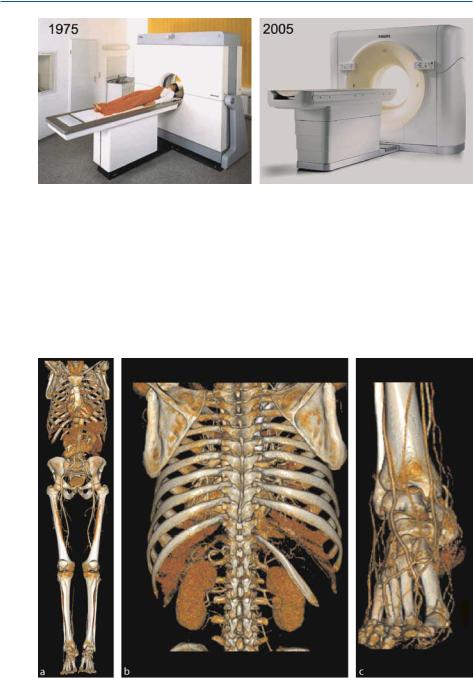
With respect to the subtitle of this book, it is structured to cover the basics of CT, from photon statistics to modern cone-beam systems. Without an elementary knowledge of X-ray physics, a number of the described imaging e ects and artifacts cannot readily be understood. In Chap. , X-ray generation, photon–matter interaction, X-ray detection, and photon statistics are briefly summarized. In Chap. , a retrospective overview of the historical milestones on the road map of the technical developments in computed tomography is given. Starting with tomosynthesis in the s and s, the di erent types or generations of CT are characterized. The chapter concludes with motivation for the modern scanner concepts like electron-beam CT (EBCT), micro-CT, and especially helical cone-beam CT. Although remarkable advances in CT technology have been achieved, Fig. . shows that the appearance of the gantry has undergone only a slight change throughout the years.
1 Introduction
Fig. . . Design of CT gantries in and (courtesy of Philips Medical Systems)
In Chap. , the principles of signal processing are reviewed. This chapter focuses on the necessary background of computed tomography and consequently uses signals of spatial variability. Chapters and give a detailed overview of two-dimensional reconstruction mathematics. The most important algorithms are derived step by step. In Chap. , the Fourier-based methods are collected. InChap. , the algebraic and statistical approaches are explained.
Fig. . a–c. Whole body scans can be performed with the latest generation of CT systems, including a multi-slice detector system. Even very small vessels of the feet can be precisely visualized (courtesy of Philips Medical Systems)
1.5 Structure of the Book |
|
In Chap. , the limitations of the practical implementation of the previously described methods are discussed. Specifically, the correspondence of the parallel pencil-beam and the fan-beam X-ray system are demonstrated.
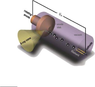
In Chap. , the three-dimensional methods of CT image or volume reconstruction are reviewed. It is shown that some of the ideas are consequent extensions of the methods discussed in Chap. . The methods described in this chapter represent the basis of a highly active field of research. A description of the existing manifold algorithmic variations in the field of helical cone-beam methods, for instance, is beyond the scope of this book. However, in Fig. . an example of the impressive quality of the three-dimensional reconstruction results of modern multi-slice CT scanners is given.
In Chap. , an introduction to the methods of image quality evaluation is given. The chapter focuses on typical artifacts of computed tomography, whereby two-dimensional and three-dimensional artifacts are di erentiated. Additionally, the important fourth power law is derived that describes the correspondence among signal-to-noise ratio, dose, and detector element size.
In Chap. , some practical aspects of computed tomography are described. This includes CT planning, which uses the overview scan mentioned previously, the mapping of the physical attenuation values to the Hounsfield scale, and a list of exemplary application fields of CT in practice. Finally, Chap. concludes the book with a review of dose issues in clinical computed tomography.

2Fundamentals of X-ray Physics
Contents
2.1 Introduction . . . . . . . . . . . . . . . . . . . . . . . . . . . . . . . . . . . . . . . . . . . . . . . . . . . . . . . 15 2.2 X-ray Generation . . . . . . . . . . . . . . . . . . . . . . . . . . . . . . . . . . . . . . . . . . . . . . . . . . . . 15 2.3 Photon–Matter Interaction . . . . . . . . . . . . . . . . . . . . . . . . . . . . . . . . . . . . . . . . . . . . . 31 2.4 Problems with Lambert–Beer’s Law . . . . . . . . . . . . . . . . . . . . . . . . . . . . . . . . . . . . . . 46 2.5 X-ray Detection . . . . . . . . . . . . . . . . . . . . . . . . . . . . . . . . . . . . . . . . . . . . . . . . . . . . . 48 2.6 X-ray Photon Statistics . . . . . . . . . . . . . . . . . . . . . . . . . . . . . . . . . . . . . . . . . . . . . . . . 59
2.1 Introduction
For the discovery of a new radiation capable of high levels of penetration, Wilhelm Conrad Röntgen was awarded with the first Nobel Prize for physics in . In , in experiments with accelerated electrons, he had discovered radiation with the ability to penetrate optically opaque objects, which he named X-rays. In this chapter, the generation of X-rays, photon–matter interaction, X-ray detection, and statistical properties of X-ray quanta will be described. However, the scope of this chapter is limited to physical principles that are relevant to computed tomography (CT). A more comprehensive description can be found in many physics text books, for example Demtröder ( ), and in overviews on radiological technology, for example Curry et al. ( ). One of the main reasons for the wide exploitation of Röntgen’s radiation was the simple equipment required for X-ray generation and detection. Nevertheless, the development of robust, high-power X-ray tubes that are optimized for use in CT, is ongoing.
2.2
X-ray Generation
X-ray radiation is of electromagnetic nature; it is a natural part of the electromagnetic spectrum, with a range that includes radio waves, radar and microwaves, infrared, visible and ultraviolet light to X- and γ-rays. In electron-impact X-ray
|
2 Fundamentals of X-ray Physics |
sources, the radiation is generated by the deceleration of fast electrons entering a solid metal anode, and consists of waves with a range of wavelengths roughly between − m and − m. Thus, the radiation energy depends on the electron velocity, ν, which in turn depends on the acceleration voltage, Ua, between cathode and anode so that with the simple conservation of energy
eUa = |
|
|
|
|
meν |
( . ) |
|
|
|||
the electron velocity can be determined. |
|
|
|
2.2.1
X-ray Cathode
In medical diagnostics acceleration voltages are chosen between kV and kV, for radiation therapy they lie between kV and kV, and for material testing they can reach up to kV. Figure . shows a schematic drawing of an X-ray
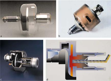
Fig. . . Schematic drawing of an X-ray tube. Thermal electrons escape from a cathode filament that is directly heated to approximately , K. The electrons are accelerated in the electric field between cathode and anode. X-ray radiation emerges from the deceleration of the fast electrons following their entry into the anode material
Charge of electrons: e = . ċ − C; mass of electrons: me = . ċ − kg.
There is no clear definition of the X-ray wavelength interval. The range overlaps with ultraviolet and γ-radiation.
Acceleration energy is measured in units called electron volts (eV). eV is the energy that an electron will gain if it is accelerated by an electrical potential of one volt. The same unit is used to measure X-ray photon energy.

2.2 X-ray Generation |
|
tube. Electrons are emitted from a filament, which is directly heated to approximately , K to overcome the binding energy of the electrons to the metal of the filament .
The binding energy, Ev, is due to two main e ects (Bergmann and Schäfer ). The first e ect is the formation of a dipole layer at the cathode surface. When a free inner electron moves toward the surface of the metal, electrostatic forces prevent the electron from escaping. However, before reversing its direction, the electron overshoots the outer metal ion layer, and, as a result, an electron is missing inside the metal for charge neutralization. The surplus of positive charge at the inner side of the surface layer, together with the negative electron outside the metal, forms an electric dipole layer. The electric field inside the dipole layer slows down electrons
trying to leave the metal. This e ect results in the part WDipole of the work function. The other part originates from what is called a mirror-image force. Due to elec-
trostatic influence, an electron above a metal surface causes a charge displacement inside the metal. The resulting electric field between the electron and the metal surface looks like the field between a charge, −e, above and a virtual mirror charge, +e, below the metal boundary at the same distance x from the boundary. To bring an electron from distance d above the surface to infinity, the work
Wmirror = |
e |
|
dx |
= |
e |
|
|
d∫ |
( x) |
|
( . ) |
||
πε |
πε d |
Fig. . . The electron beam is controlled by a cylindrically shaped electrode, containing the cathode with opposite potential. This electron optics is called a Wehnelt cylinder, or is sometimes also called a focusing cup. In this way, the electrons are steered onto a small focal point on the anode. Shown in a is a dual-filament and in b a modern mono-filament; both are designed to produce focal spot sizes of . mm and . mm (courtesy of Philips Medical Systems)
Filaments are usually made of thoriated tungsten with a melting point at , C.

|
2 |
|
Fundamentals of X-ray Physics |
|
|||
|
must be applied. Since the metal–vacuum interface is not an ideal mirror surface, it |
||||||
|
is sensible to start the integration at a distance of approximately one atom diameter |
||||||
|
(d |
− m), leading to a work of Wmirror |
. eV. |
||||
|
|
|
Due to their thermal energy, electrons are boiled o from the filament. This |
||||
|
process is called thermionic emission. The temperature of the metal must be high |
||||||
|
enough to increase the kinetic energy, Ekin, of the electrons such that Ekin |
||||||
|
E |
v |
|
Wdipole |
|
|
- |
|
|
= |
+ |
Wmirror. The emission current density, je, is essentially a func |
|||
|
|
|
|
|
|
||
Fig. . . Simulation of electron trajectories emitted from the filament and accelerated onto the anode. The potential at the Wehnelt cylinder controls the electron focus on the anode. Below: Shape and size of a large and a small X-ray focus (courtesy of Philips Medical Systems)

2.2 X-ray Generation |
|
tion of the temperature and can be described by the tion
je = CRD T e− kφT ,
where CRD is the Richardson–Dushman constant
= πme k e CRD h ,
Richardson–Dushman equa-
( . )
( . )
k is the Boltzmann constant and φ is the work function defined as the di erence between Ev and the Fermi energy edge. An electron cloud forms around the filament and these electrons are subsequently accelerated toward the anode. When the electrons reach the surface of the anode they will be stopped abruptly.
To produce a small electron focus on the anode, the trajectories of the accelerated electrons must be controlled by electron optics. The focusing device can be seen in Fig. . . Basically, it is a cup-shaped electrode that forms the electric field near the filaments such that the electron current is directed to a small spot. In Fig. . it can be seen how the potential of the Wehnelt optics (frequently named Wehnelt cylinder) influences the electron trajectories. In this way, the cylinder can easily be controlled to produce a large or small X-ray focus. The e ect that this has on imaging quality will be discussed in a later section.
2.2.2
Electron–Matter Interaction
With the entry of accelerated electrons into the anode, sometimes also called the anticathode, several processes take place close to the anode surface. Generally, the electrons are di racted and slowed down by the Coulomb fields of the atoms in the anode material. The deceleration results from the interaction with the orbital electrons and the atomic nucleus. As known from classical electrodynamics, acceleration and deceleration of charged particles creates an electric dipole and electromagnetic waves are radiated. Usually, several photons emerge throughout the complete deceleration process of one single electron. Figure . a illustrates two successive deceleration steps. It can happen, however, that the entire energy, eUa, of an electron is transformed into a single photon. This limit defines the maximum energy of the X-ray radiation, which can be determined by
eUa |
|
hνmax |
|
Emax . |
( . ) |
The limit Emax corresponds to the |
minimum wavelength |
|
|||
= |
|
= |
|
|
|
|
|
|
|
λmin |
|
|
hc |
|
. nm |
, |
||
|
|
|
|
=−eUa |
= |
|
||||||
|
|
|
|
|
Ua kV |
|||||||
|
For ideal metals CRD |
|
− |
|
|
|||||||
|
|
A cm |
|
K |
. However, in practice CRD |
|||||||
|
|
|
= . ċ |
− |
|
− |
. |
|
|
|
||
|
Boltzmann constant: k |
|
|
J K |
|
|
|
|||||
. eV for tungsten.
( . )
is material-dependent.
|
2 Fundamentals of X-ray Physics |
Fig. . . X-ray spectrum of a tungsten anode at acceleration voltages in the range of Ua = –kV. The anode angle is and mm Al filtering has been applied. The intensity versus wavelength plot shows the characteristic line spectrum as well as the continuous bremsstrahlung (courtesy of B. David, Philips Research Labs). The minimum wavelength is determined by the total energy, eUa, of the electron reaching the anode. Process illustrations: a bremsstrahlung, b characteristic emission, c Auger process and d direct electron-nucleus collision
where h is Planck’s constant and c is the speed of light . While the acceleration voltage determines the energy interval of the X-ray spectrum, the intensity of the generated X-ray spectrum or the number of X-ray quanta, is solely controlled by the anode current.
Planck’s constant: h = . ċ − Js; speed of light in vacuum: c = . ċ m s.

|
|
|
|
|
|
|
|
|
|
|
|
|
|
|
|
2.2 |
X-ray Generation |
|
|||
Due to the fact that the slowing down of electrons in the anode material is |
|
||||||||||||||||||||
a multi-process deceleration cascade, a continuous distribution of energies can be |
|
||||||||||||||||||||
shown by the bremsstrahlung (cf. Fig. . ). Since the free electrons are unbound, |
|
||||||||||||||||||||
their energy cannot be quantized. The energy balance can be described by the fol- |
|
||||||||||||||||||||
lowing equation |
|
|
|
|
|
|
|
|
|
|
|
|
|
|
|
|
|
|
|
||
E |
kin |
e− |
|
atom lattice |
|
|
|
atom lattice |
E |
kin−h |
ν |
|
e− |
|
|
hν . |
( . ) |
|
|||
|
|
|
|
|
|
|
|
|
|
|
|
|
|
|
|
|
|
|
|
||
|
|
|
process of X-ray generation by electron deflection is a rare one. |
|
|||||||||||||||||
Unfortunately,(the)(+ |
|
) ( |
|
|
|
|
+) |
|
|
( |
|
) + |
|
|
|
||||||
It has been shown (Agawal ) that the intensity of bremsstrahlung follows |
|
|
|||||||||||||||||||
|
|
|
|
I |
|
Zh |
|
|
νmax |
|
ν |
, |
|
|
|
|
|
|
|
( . ) |
|
where Z is the atomic number of the |
anode material. The conversion e ciency from |
|
|||||||||||||||||||
|
( |
|
− |
) |
|
|
|
|
|
|
|
|
|
|
|||||||
kinetic electron energy to bremsstrahlung energy can be described by |
|
|
|||||||||||||||||||
|
|
|
|
|
η = KZUa , |
|
|
|
|
|
|
|
|
|
( . ) |
|
|||||
where K is a material constant that was found by Kramers ( ) to theoretically be K = . ċ − kV− when the acceleration voltage, Ua, is given in kV.
The continuous bremsstrahlung is superimposed by a characteristic line spectrum, which originates from direct interaction of fast electrons with the inner shell electrons of the anode material. If an electron on the K-shell or K-orbital is kicked out of the atom by a collision with a fast electron, i.e., the atom is ionized by the loss of an inner electron, an electron of one of the higher shells fills the vacant position on the K-shell. An example for the energy balance of the transition of an L-electron to the K-shell is given by
EK(Atom+) EL(Atom+) + hνKL . |
( . ) |
As the inner shells represent states having a lower potential energy than the outer shells, this process is accompanied by the emission of a photon. Due to the highenergy di erence between the inner shells, these photons, with a wavelength
λ = |
hc |
( . ) |
Ei − Ej |
are X-ray quanta. This process creates sharp lines in the X-ray spectrum that are characteristic finger prints for the anode material. The notation of these lines is agreed upon as follows: Kα , Kβ , Kγ , ... denote the transition of an electron from the L-, M-, N-, ... shell to the K-shell and Lα , Lβ, Lγ, ... denote the transition from the M-, N-, O-, ... shell to the L-shell, etc. Figure . b illustrates a Kβ emission.
The position of the characteristic K-line spectrum is given by Moseley’s Law
λ = |
hc |
= |
hc |
|
|
|
|
, |
( . ) |
||
En − E |
. eV(Z − ) ( − n ) |
||||
where Z is again the atomic number of the anode material and n is the principal quantum number of the electron falling to the K-shell.
Experiments are in good agreement with Kramers’ result, but show a slight dependence on Z.

2 Fundamentals of X-ray Physics
The result is the production of a large number of X-ray quanta at a few discrete energies. It can be seen in Fig. . that the probability of X-ray quanta emerging by the Kα process is higher than the probability of bremsstrahlung quanta at the same energy. However, in total the characteristic X-ray radiation contributes far less to the total intensity than the bremsstrahlung. Figure . shows a typical spectrum for a tungsten anode at acceleration voltages between Ua = kV and kV. In Fig. . c a competing process, named the Auger process, is illustrated as well. Instead of emitting the Kβ radiation the atom may absorb the photon by emitting another electron, called an Auger electron. This is seen as a non-radiative process. The emerging Auger electrons are mono-energetic.
The probability of the Auger process is constant for all elements. However, the probability of emitting characteristic radiation is given by the ratio
= Z = <
P Z + a + Za ,
where a is a positive constant . For elements with low atomic numbers, the Auger process dominates, whereas for heavy elements, characteristic emission dominates.
The direct collision of the fast electron with the nucleus of an anode atom is indicated in Fig. . d. This interaction represents an ideal conversion of the entire kinetic energy of the electron to bremsstrahlung in one single deceleration process. Obviously, the collision contributes to the upper limit of the X-ray spectrum. However, from the X-ray intensity at the upper energy limit of the spectrum, it can be concluded that direct collision is a very rare interaction process. The mean energy
lost of the electron in matter can quantitatively be described by |
|
|
|
|
||||||||||||||||||||||||||||||
|
|
|
|
|
|
dE |
|
|
dE |
|
|
|
|
|
|
|
|
|
|
|
dE |
|
|
|
|
, |
|
|
|
( . ) |
||||
|
|
|
|
|
|
dx |
|
|
dx |
|
|
|
|
|
|
|
|
|
|
|
|
dx |
|
|
|
|
|
|
|
|||||
|
|
|
|
|
|
|
|
|
bremsstrahlung |
|
|
|
ionization |
|
|
|
|
|||||||||||||||||
where the first |
term of ( . ) is given by quantum electrodynamics (QED) |
|
|
|||||||||||||||||||||||||||||||
|
|
|
= |
|
|
|
|
|
|
|
+ |
|
|
|
|
|
|
|
|
|
|
|
|
|||||||||||
|
|
|
dE |
|
|
|
|
|
|
|
|
|
|
|
|
Z |
|
|
e |
|
|
|
|
|
|
|
|
|
|
|||||
|
|
|
|
|
|
|
|
|
αN |
|
ρ |
|
|
|
E ln |
|
|
, |
( . ) |
|||||||||||||||
|
|
|
|
|
|
|
|
|
|
|
|
|
A me c |
Z |
|
|||||||||||||||||||
|
|
dx bremsstrahlung = − |
A |
|
|
|
|
|
|
|||||||||||||||||||||||||
where α is the fine-structure constant |
, Z is the atomic number, ρ is the density, |
|||||||||||||||||||||||||||||||||
A is the atomic weight of the material, and NA is the Avogadro constant . |
|
|
||||||||||||||||||||||||||||||||
|
The second term of ( . ) is given by the Bethe–Bloch equation |
|
|
|
||||||||||||||||||||||||||||||
|
dE |
|
|
|
|
|
Z |
|
e |
z |
|
|
|
m |
e |
c β γ T |
|
|
δ |
|||||||||||||||
|
ionization |
= − πNA ρ |
|
|
|
|
|
|
|
|
ln |
|
|
|
|
|
max |
|
− β − |
|
. |
|||||||||||||
dx |
A |
me c |
β |
|
|
|
|
|
I |
|
|
|
|
|||||||||||||||||||||
( . )
The electron velocity is given in units of the speed of light, i.e., β = v c, and, here, the charge of the electron z is given in units of the elementary charge, therefore, z = . γ is the Lorentz factor, i.e., γ = ( − β )− . Tmax is the maximum kinetic energy to be transferred in a single collision. I is the mean ionization energy of the material and δ is a density correction of the ionization energy.
For K-shell emission a = . ċ (Otendal ). Fine-structure constant: α = e ( πε ħc) . . Avogadro constant: NA = . ċ mol− .
2.2 X-ray Generation |
|
2.2.3 Temperature Load
Using ( . ), it can be estimated that the quantum e ciency of the conversion from kinetic energy into X-ray radiation, within a tungsten anode (W, Z = ), and working with an acceleration voltage of Ua = kV, is roughly in the magnitude of η = . . This means that % of the kinetic energy is transferred locally to the lattice, heating up the anode. As a result, CT X-ray tubes have serious heat problems. Since it is the energy deposition in the target volume that produces the heat load, the tube current and the duration of exposure or, more precisely, the product of current in milliamperes and exposure time in seconds, are two important parameters of the practical scan protocol the radiologist has to choose appropriately. The heat capacity of an X-ray tube is measured in Heat Units
HU = U ċ I ċ t . |
( . ) |
For several decades rotating anode disks have been used to distribute the thermal load over the entire anode. The anode target material is rotated about the central axis and therefore, new, cooler anode material is constantly rotated into position at the focal spot (Mudry ). In this way, the energy of the electron beam is spread out over a line, called the focal line, rather than being concentrated at one single
Fig. . a–d. X-ray tubes through the years a , b , c , and d schematic illustration of a modern X-ray tube with a rotating anode disk (courtesy of Philips Medical Systems)

|
2 Fundamentals of X-ray Physics |
Fig. . . a X-ray anode with b spiral-groove bearing (courtesy of Philips Medical Systems)
point. This line focus principle was invented in , and in the idea of a rotating anode was realized (Otendal ). Figure . shows di erent types of CT X-ray tubes with rotating anode disks that have been used down the years. In Fig. . a a tube from is shown. It was integrated into single-slice CT with a scan time of s per slice. The heat capacity was – HU. In , an X-ray tube with a heat capacity of – HU came onto the market (Fig. . b). This tube was ready to be integrated into spiral-CT systems. In Fig. . c a modern tube that is used today is shown. It has a heat capacity of – HU and has been integrated into recent multi-slice CT systems. A significant part of the heat (about %) is conducted via the bearing of the rotating anode as schematically drawn in Fig. . d. The rest of the heat is transferred via radiation to the housing of the X-ray tube. The rotation frequency is very high, causing mechanical parts of the tube to be subjected to g-forces of up to g. A liquid metal-filled spiral-groove bearing as shown in Fig. . allows very high continuous power compared with conventional ball bearings. Often, a heat exchanger is placed on the rotating acquisition disk to cool the anode.
For the design of an optimal X-ray tube anode it has been found that a material with high e ciency, i.e., a large Z, high thermal conductivity, λt, and a maximum melting point temperature, ϑmax, must be chosen. For rotating anodes Zϑmax(λt ρc) must be optimized, where ρ is the mass density and c the heat capacity. Tungsten fulfills these requirements (Morneburg ).
2.2.4
X-ray Focus and Beam Quality
Ideally, X-rays should be created from a point source, because an increase in source size will result in a penumbra fringe in the image of any object point. The size and shape of the X-ray focus seen by the detector determines the quality of the resulting

2.2 X-ray Generation |
|
image. The e ective target area, called the optical focus, depends on the orientation of the anode surface that is angulated with respect to the electron beam. The projection of the focus shape onto the detector must be minimized to obtain a sharp image. However, this surface angle increases the tube power limit, because it allows the heat to be deposited across a relatively large spot while the apparent spot size at the detector will be smaller by a factor of the sine of the anode angle (Mudry ).
Figure . schematically illustrates that the image quality is degraded by a large focus diameter, due to significant partial shadow areas of each object point. The mathematical expression that measures the image quality is called the modulation transfer function (MTF). Mathematical measures of image quality will be discussed in detail in Chap. . A large angle between the incident electron beam and the anode surface normal is generally not desired because there is a certain probability that the electrons are elastically reflected from the surface and thus do not contribute to X-ray generation. The probability of this backscattering e ect increases as the atomic number of the anode material increases and as the angle between the surface normal and the anode rotation axis decreases.
Fig. . a–c. The size of the optical focal point is determined by the orientation of the anode surface normal relative to the electron beam. The larger the optical focal point, the more blurred the image becomes, since all points of the object are surrounded by a penumbra fringe
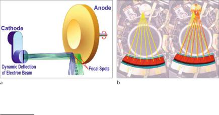
|
2 Fundamentals of X-ray Physics |
|||
|
Typically, the X-ray focus diameter for diagnostic tubes is found to be between |
|||
|
. mm and mm. The penetration depth of electrons into the anode depends on |
|||
|
the kinetic energy and the anode material and can be found up to μm. The radi- |
|||
|
ologist may have the option of choosing between two focus sizes. This is technically |
|||
|
realized by focusing the electron beam onto two target points with di erent anode |
|||
|
orientations. Figure . illustrates that the spatial resolution of the detector can also |
|||
|
be doubled by switching between two foci during data acquisition. This concept is |
|||
|
called a flying focus. |
|||
|
The basic assumption of the imaging principles of fluoroscopy and of CT recon- |
|||
|
struction is that the object to be scanned is illuminated homogeneously. Therefore, |
|||
|
another factor that must be considered regarding image quality is the directional |
|||
|
characteristic of the X-ray. Slight deviations from a homogeneous beam profile can |
|||
|
be compensated for by specially formed filters mounted on the X-ray tube and by |
|||
|
detector calibration. The next paragraphs give a brief explanation of the physical |
|||
|
mechanism that leads to inhomogeneous object illumination. |
|||
|
Generally, two e ects are responsible for a directional characteristic of the ef- |
|||
|
fective X-ray beam. As discussed above, bremsstrahlung is produced by dipole radi- |
|||
|
ation that shows the specific Hertzian antenna characteristic. Fast electrons acceler- |
|||
|
ated with Ua |
|
kV have a velocity of roughly % of the speed of light, meaning |
|
|
that |
relativistic e ects emerge. In the case of dipole radiation, the relativistic model |
||
|
|
= |
|
|
reveals an antenna characteristic that points into the same direction as the electron velocity. This relativistic e ect grows with increasing kinetic energy of the electrons. In Fig. . a the antenna characteristic for a relativistic dipole is shown. However, with respect to the total radiation characteristic of the X-ray tube, this e ect is less important because, as mentioned above, bremsstrahlung is produced in a multiple deceleration cascade. Since the direction of the electron changes with each deceleration step, in practice, the radiation is homogeneous over π. For this reason, X-ray
Fig. . a,b. With a flying focus the spatial resolution of the sampling unit can be doubled
The diameter of the X-ray focus depends on the diagnostic application (see for example Huda and Slone [ ]).
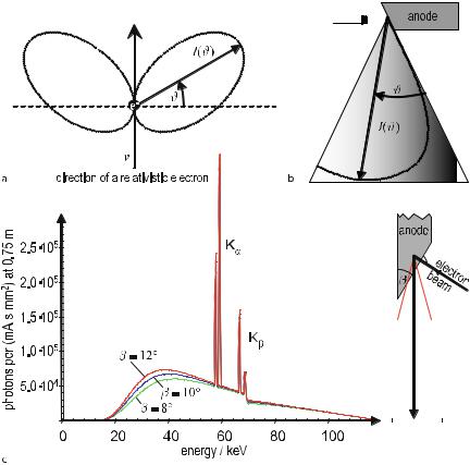
|
|
|
|
2.2 X-ray Generation |
|
||||||||
|
|
|
|
|
|
|
|
|
|
|
|
|
|
|
|
|
|
|
|
|
|
|
|
|
|
|
|
|
|
|
|
|
|
|
|
|
|
|
|
|
|
|
|
|
|
|
|
|
|
|
|
|
|
|
|
|
|
|
|
|
|
|
|
|
|
|
|
|
|
|
|
|
|
|
|
|
|
|
|
|
|
|
|
Fig. . . a Radiation directionality of a Hertz dipole producing bremsstrahlung during relativistic electron deceleration. b Heel e ect: Intensity reduction of X-ray due to self absorption at the anode surface. c X-ray spectra of a tungsten anode simulated for di erent anode angles at Ua = kV and mm Al filtering (courtesy of B. David, Philips Research Labs)
tubes have a protective housing with a window for the useful beam; otherwise theπ characteristic would cause the patient and the radiologist to be exposed to an unnecessary dosage.
More important than the relativistic e ects are the surface e ects of the anode. X-ray beams leaving the anode tangential to the anode surface are reduced in intensity when arriving at the detector. This intensity reduction is due to the selfabsorption of photons by the anode, caused by the microscopic roughness of the anode surface. In Fig. . b the characteristic of X-ray intensity versus radiation direction is schematically illustrated. The X-ray intensity decreases gradually with a reduction in the angle, ϑ, between beam and anode surface. This e ect, which is called the Heel e ect, grows during the lifetime of any X-ray tube, because the roughness of the anode surface increases (see Fig. . ) due to erosion by electron bombard-

|
2 Fundamentals of X-ray Physics |
Fig. . . a Appearance of a used anode disk after , scans. b–d Di erent magnifications of the focus lines. The surface shows - to -mm-deep cracks and a loss of grains (courtesy of Philips Medical Systems)
ment along the focus line (Heinzerling ). Figure . c shows the resulting X-ray spectra simulated for a tungsten anode at an acceleration voltage of Ua = kV and mm Al beam filtering. It can be seen that the X-ray intensity decreases with the anode angle, β, especially for lower energy X-rays, due to the self absorption process.
However, in modern CT systems the cone of the utilized X-rays is becoming larger and larger. Therefore, it is important to know the radiation characteristics of the anode.
2.2.5
Beam Filtering
It should be noted at this point, that the image quality of CT specifically su ers from the fact that attenuation is a complicated function of the wavelength. The details of the functional behavior are given in the next section. Generally, one has to bear in mind that a low-energy X-ray, i.e., radiation with a larger wavelength, is

2.2 X-ray Generation |
|
more strongly attenuated when passing through matter than high-energy X-ray . As a consequence, the center of the polychromatic X-ray is shifted to higher energies or harder radiation respectively. This is the origin of what is called beam hardening, which produces artifacts in the reconstructed images, because today it is standard to
Fig. . . Beam hardening of an X-ray spectrum produced by a tungsten anode (anode angle, acceleration voltage Ua = kV) due to filtering by a flat, . -mm source side-mounted aluminum filter and a . -mm copper filter respectively. The amount of intensity reduction depends on the wavelength. The intensity of the high-energy bremsstrahlung of the copperfiltered spectrum is even higher than the intensities of the characteristic Kα and Kβ lines (courtesy of B. David, Philips Research Labs)
Low energy quanta are generally undesired in X-ray imaging. They increase the dose to the patient, but do not contribute to imaging, because they are almost totally absorbed by the human body.
|
2 Fundamentals of X-ray Physics |
|||||||||||||||||||||||
|
consider the X-ray to be monochromatic within the mathematical reconstruction |
|||||||||||||||||||||||
|
process. |
|||||||||||||||||||||||
|
|
Artifacts due to beam hardening will be discussed in Sect. . . . In Fig. . the |
||||||||||||||||||||||
|
|
|
|
|
|
|
|
|
|
|
|
|
|
|
|
|
hardening is demonstrated |
|||||||
|
X-ray spectrum of a tungsten anode is shown. The beam |
|||||||||||||||||||||||
|
by a source side aluminum and copper filter respectively. Generally, a flat metal filter |
|||||||||||||||||||||||
|
measuring a few millimeters is mounted to the X-ray tube. The filtering of the useful |
|||||||||||||||||||||||
|
beam reduces the number of X-ray quanta while increasing the average energy of |
|||||||||||||||||||||||
|
the radiation. This pre-hardening of the radiation reduces beam-hardening artifacts |
|||||||||||||||||||||||
|
during image reconstruction and the dose to which the patient is exposed. |
|||||||||||||||||||||||
|
2.2.6 |
|
|
|
|
|
|
|
|
|
|
|
|
|
|
|
|
|
|
|
|
|
||
|
Special Tube Designs |
|||||||||||||||||||||||
|
Although much e ort has been made to increase the heat capacity of X-ray tube |
|||||||||||||||||||||||
|
anodes, the power of these tubes is still limited. Since there is a desire for higher |
|||||||||||||||||||||||
|
power tubes that are also of lower weight, specially designed X-ray devices have re- |
|||||||||||||||||||||||
|
cently been developed. One design abandons the solid-state principle of the anode. |
|||||||||||||||||||||||
|
In these tubes a liquid metal jet is subjected to fast electrons. The main idea is very |
|||||||||||||||||||||||
|
simple. Liquid metal, eutectics of SnPb, GaInSn, or PbBiInSn, turbulently stream- |
|||||||||||||||||||||||
|
ing through a tube close to the cathode, is heated at the focal spot. While the heated |
|||||||||||||||||||||||
|
|
|
|
|
|
|
|
|
|
|
|
|
|
|
|
|
|
|
|
|
|
|
|
|
|
|
|
|
|
|
|
|
|
|
|
|
|
|
|
|
|
|
|
|
|
|
|
|
|
|
|
|
|
|
|
|
|
|
|
|
|
|
|
|
|
|
|
|
|
|
|
|
|
|
|
|
|
|
|
|
|
|
|
|
|
|
|
|
|
|
|
|
|
|
|
|
|
|
|
|
|
|
|
|
|
|
|
|
|
|
|
|
|
|
|
|
|
|
|
|
|
|
|
|
|
|
|
|
|
|
|
|
|
|
|
|
|
|
|
|
|
|
|
|
|
|
|
|
|
|
|
|
|
|
|
|
|
|
|
|
|
|
|
|
|
|
|
|
|
|
|
|
|
|
|
|
|
|
|
|
|
|
|
|
|
|
|
|
|
|
|
|
|
|
|
|
|
|
|
|
|
|
|
|
|
|
|
|
|
|
|
|
|
|
|
|
|
|
|
|
|
|
|
|
|
|
|
|
|
|
|
|
|
|
|
|
|
|
|
|
|
|
|
|
|
|
|
|
|
|
|
|
|
|
|
|
|
|
|
|
|
|
|
|
|
|
|
|
|
|
|
|
|
|
|
|
|
|
|
|
|
|
|
|
|
|
|
|
|
|
|
|
|
|
|
|
|
|
|
Fig. . . a Basic principle of the liquid metal X-ray tube. b The anode module consists of
aconstricted fluid channel incorporating an exchangeable electron-beam window module. c The anode module itself is connected to a fluid circuit containing a displacement pump and
awater-cooled cross-flow heat exchanger. d Infrared imaging of the focal spot temperature (courtesy of Philips Research, Hamburg [David et al. , ])
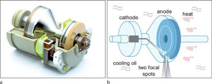
2.3 Photon–Matter Interaction |
|
Fig. . a,b. Straton design: Directly cooled StratonTM X-ray tube with alternating focal spots (courtesy of Siemens Medical Solution)
material is transported through the tubing, cold metal enters the focal spot area. A schematic diagram of what is known as the LIMAX tube (Liquid Metal Anode X-ray) is shown in Fig. . . The liquid metal is cooled e ectively by circulation through a heat exchanger. The liquid metal is separated from the vacuum by a diamond, tungsten or molybdenum window of several microns in thickness (David et al. , ). In comparison to stationary anode X-ray tubes, the LIMAX design has shown a significant improvement in its ability to be continuously loaded. However, in the current state of development, the peak power does not reach values, to the order of kVA, that are required for the latest CT generation.
A di erent strategy for direct tube cooling is implemented by the Straton X-ray tube (see Fig. . a,b). The direct anode cooling, realized by completely embedding the rotating housing in cooling oil, eliminates the need for heat storage capacity and therefore permits a smaller tube size. Thanks to its low weight, this kind of X-ray device has been integrated into the current state-of-the-art dual source generation of CT scanners.
2.3
Photon–Matter Interaction
The X-ray is known to have a very high, material-dependent capability of matter penetration. However, the number of photons, i.e., the radiation intensity, decreases exponentially while running through an object along the incident direction. This attenuation is due to absorption and scattering. The reason for an exponential reduction in photon number is that each photon is removed individually from the incident beam by an interaction. In this chapter, the most important physical mechanisms of photon–matter interaction (i.e., Rayleigh scattering, Compton scattering, photoelectric absorption, and pair production), as well as their mathematical models, will be explained briefly.
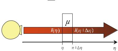
|
2 Fundamentals of X-ray Physics |
|
2.3.1 |
|
Lambert–Beer’s Law |
As illustrated in Fig. . , all physical mechanisms that lead to the attenuation of radiation intensity (reduction of photons) measured by a detector behind a homogeneous object are usually to be subsumed by a single attenuation coe cient, μ. Within this simple model the total attenuation of a monochromatic X-ray beam can be calculated in the following way. The radiation intensity – which is proportional to the number of photons – after passing a distance η through an object is determined by
I(η + η) = I(η) − μ(η)I(η) η . |
( . ) |
By simple reordering of ( . ) the quotient
I |
( |
η |
+ |
η |
) − |
I |
( |
η |
) = − ( ) ( ) |
|
|
|
|
|
|
|
|
|
|
|
|
μ η I η |
( . ) |
η
can be obtained. Taking the limit of ( . ) leads to the di erential quotient
|
|
I |
( |
η |
+ |
η |
) − |
I |
( |
η |
) = |
dI |
= − |
|
( |
|
) |
( |
|
) |
|
|
|
lim |
|
|
|
|
|
η |
|
|
|
|
|
dη |
|
μ |
|
η |
I |
|
η |
|
. |
( . ) |
|
η |
|
|
|
|
|
|
|
|
|
|
|
|
|
|
|
|
|
|
|
|
|
|
|
In a first step, the medium is assumed to be homogeneous, i.e., in ( . ) the object can be described by a single attenuation constant μ(η) μ along the entire length of penetration. This leads to an ordinary linear and homogeneous, firstorder di erential equation with constant coe cients. The solution is obtained by separation of variables. Consider the right-hand side of ( . ), which can be separated to
dI |
|
I(η) = −μ dη . |
( . ) |
Fig. . . Mathematical model of monochromatic X-ray attenuation. The photons are running through an object of thickness η with a constant attenuation coe cient, μ. Equal parts of the same absorbing medium attenuate equal fractions of the radiation

|
|
|
|
2.3 Photon–Matter Interaction |
|
Integration of both sides of ( . ) |
|
|
|
||
|
∫ |
dI |
= −μ ∫ dη |
( . ) |
|
gives |
I(η) |
|
|||
|
ln I |
μ η C . |
( . ) |
|
|
Due to the physical fact that the intensity= −is defined+ |
as a positive quantity, the abso- |
|
|||
lute sign, ċ , is obsolete so that subsequent exponentiation leads to |
|
||||
|
I(η) = e−μη+C . |
( . ) |
|
||
With the initial condition I( ) = I , the special solution of the di erential equation ( . )
I(η) = I e−μ η , |
( . ) |
is obtained, known as Beer’s law of attenuation . The linear attenuation coe - cient, μ, of ( . ) is an additive combination of a scatter coe cient, μs, and an absorption coe cient, α, i.e.,
μ = μs + α . |
( . ) |
The attenuation coe cient is measured in units of [μ] = m− . Beer’s law holds for pencil-beam geometry only, where the scattered radiation is completely removed from the main beam. With a wide beam, much of the scattered radiation carries on with a forward component to its direction (Barrett and Swindell ). Generally, the linear attenuation coe cient is given by
μ = |
ρNA |
ċ σtot = n ċ σtot , |
( . ) |
A |
where ρ is again the density, A is the atomic weight of the material and NA is the Avogadro constant. That means the attenuation coe cient is given by the number of target atoms per unit volume, n, times the total photon atomic cross-section, σtot, for either scattering or absorption.
By introducing the absorber density, ρ, the mass attenuation coe cient
κ = μ ρ |
( . ) |
can be defined. The mass attenuation coe cient is measured in units of [κ] = m kg. This coe cient is useful for estimating the mass of a material required to attenuate the primary beam in the design of X-ray shielding.
This observation holds for monoenergetic X-ray. In the case of polychromatic X-ray one must integrate over all energies.

|
2 Fundamentals of X-ray Physics |
2.3.2
Mechanisms of Attenuation
In the following paragraphs the principal individual competing physical processes modeled by ( . ) will be explained briefly. Generally, photon interaction can result in a change in incoming photon energy and/or photon number and/or traveling direction. In Fig. . , the single processes are summarized schematically.
2.3.2.1
Rayleigh or Thomson Scattering
Rayleigh or Thomson scattering is an elastic scattering event that can be observed if the diameter of the scattering nucleus is small compared with the wavelength of the incident radiation. The incident and the scattered X-ray have equal wavelength, but the directions of the scattered rays are di erent from those of the incident beam. Consequently, there is no energy transfer. The cross-section can be derived by the classical model in which the electric field of the incoming beam drives strongly bound electrons of an atom up and down. This makes the electrons radiate
– again, as in the case of the emergence of bremsstrahlung discussed in Sect. . . , due to their acceleration – during oscillation, creating a dipole. The Thomson crosssection (Feynman ) is given by
|
σThomson |
= |
|
πre |
|
ω |
|
( . ) |
||
where |
|
|
|
(ω − ω ) |
|
|||||
|
|
|
|
|
||||||
|
re = |
|
|
|
|
e |
|
|
( . ) |
|
|
πε mec |
|
||||||||
is the classical electron radius and, ε is the permittivity of free space . |
|
|||||||||
Principally, at low energies (ω < ω , with ω being the natural frequency of the bounded atom electrons) elastic scattering is an important part of attenuation
because the probability of scattering is proportional to the th power of the radiation frequency . However, at very high frequencies ω ω , the Thomson crosssection becomes constant and competing processes become dominant . T homson, or Rayleigh, scattering is a coherent process by which photons interact with atomic bound electrons, leaving the target atoms neither excited nor ionized. Obviously,
The scattering process is called Rayleigh scattering if the momentum transferred by the photon is small compared with the momentum of the electron in the atom. In this case one must sum the amplitudes of the X-rays scattered by all electrons in the atom (see Sergé [ ]).
The scattering processes is often called Thomson scattering if it is a photon–nucleus interaction.
Permittivity of free space: ε = . ċ − F m. T his is the reason why the sky appears blue.
Therefore, coherent scattering is of less interest in classical CT. However, it has been shown recently that coherent scattering can be used for bone characterization.
2.3 Photon–Matter Interaction |
|
Fig. . . Principles of photon–matter interaction. For the Rayleigh process the dipole antenna characteristic is illustrated. For pair production the successive process of pair annihilation is illustrated as well
the model does not take into account the quantum aspects of light and, therefore, for energies being considered here, this classical scattering model yields results in disagreement to what is found by experiments.

|
2 Fundamentals of X-ray Physics |
|
|
|
||
|
There are three further mechanisms of X-ray attenuation that take the quantum |
|||||
|
mechanical interaction principles into account. These are either pure photon ab- |
|||||
|
sorption processes (photoelectric absorption and pair production) or a mixture of |
|||||
|
scattering and photo energy absorption (Compton scattering). |
|
||||
|
2.3.2.2 |
|
|
|
|
|
|
Photoelectric Absorption |
|
|
|
||
|
The entire energy of an X-ray photon, hν, can be absorbed by an atom, if the binding |
|||||
|
energies of atomic electrons are smaller than hν. The interacting electron is raised |
|||||
|
to a state of the continuous spectrum, i.e., the electron of a lower shell is kicked |
|||||
|
o the atom and travels through the material as a free photoelectron. The energy |
|||||
|
balance of this ionizing process is given by |
|
+ Ekin(e−) . |
|
||
|
hν (+ Atom) Eion(Atom+) |
( . ) |
||||
|
( . ) means that the electron leaves the atom with a kinetic energy equal to the |
|||||
|
di erence between the quantum energy of the incident photon and the binding |
|||||
|
energy of the electron. This energy di erence is removed from the primary beam |
|||||
|
and transferred locally to the lattice in the form of heat. The vacancy left by the |
|||||
|
electron that was kicked out is filled by electrons from outer shells or, in the case |
|||||
|
of solids, by electrons from the band. As a result of recombination, characteristic |
|||||
|
X-ray fluorescence lines can be measured. If the radiation energy of the successive |
|||||
|
recombination process for the electron vacancy described by ( . ) is large enough |
|||||
|
to kick out another electron in the more outlying shells, the new free electron is |
|||||
|
called an Auger electron. As mentioned already in |
Sect. . . , Auger electrons are |
||||
|
monoenergetic particles. This process is sometimes called radiation-free transition |
|||||
|
or internal conversion. |
|
|
|
||
|
The linear absorption coe cient depends on the energy, hν, of the incident |
|||||
|
X-ray beam and the atomic number, Z, of the absorber material. It has been demon- |
|||||
|
strated experimentally that a useful rule of thumb is given by |
|
||||
|
α = k |
ρ |
Z |
|
|
|
|
|
(hν) , |
|
( . ) |
||
|
A |
|
||||
where k is a constant that depends on the shell involved, ρ is the density, and A is the atomic weight of the material. Thus, the absorption is given by
α Z λ . |
( . ) |
This strong Z dependence of the absorption coe cient is utilized within the choice of radio-opaque contrast media based on for example iodine (I, Z = ) or barium (Ba, Z = ) (Lauenberger and Lauenberger ). In Fig. . the attenuation
For recovering the nature of the photoelectric absorption in , Albert Einstein received the Nobel Prize for physics in .
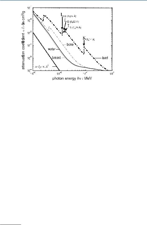
2.3 |
Photon–Matter Interaction |
|
Fig. . . Mass attenuation coe cient (α ρ measured in units of cm /g) for lead and water as well as for the bio-tissues bone and soft tissue given versus the incident radiation energy. For absorption processes above the K-shell the curve shows a fine structure (compiled with data from the web database XCOM [Berger et al. ])
=
It can be seen that ( . ) is a
coe cients are given for lead (Pb, Z ), water (H O), and two bio-materials. piecewise function for lead. However, for water and
bio-materials the functional dependence of the attenuation coe cient in the diag-
nostically relevant photon-energy interval ( keV |
|
hν |
|
keV) becomes more |
|||
complicated. |
|
|
|
|
|
||
Due to ( . ), lead (Pb, Z |
|
) shields X-ray radiation approximately , |
|||||
|
(Al, Z ). It must be noted that the mass attenu- |
||||||
times better than aluminum |
|
= |
shows a κ Z |
dependency only, because the |
|||
ation coe cient, κ, defined by ( . ) = |
|
||||||
atomic weight, A, is proportional to the atomic number, Z (Demtröder ).
If the mass attenuation coe cient is considered as a function of the incident radiation wavelength, a complicated structure is revealed. In Fig. . it can be seen that the absorption curve for lead exhibits characteristic absorption edges.
To understand the absorption edges at λk (k = , , . . .), excitation energies belonging to the wavelengths must be discussed. For wavelengths λ λk, the energy of the X-ray beam is high enough to excite an electron from an inner shell, i.e., to lift up the electron to the energy continuum, or ionize the atom. However, for wavelengths λ λk, the photon energy is too small to lift the electron to an excited, quantum mechanically allowed state. Therefore, at this very edge, the penetrated material suddenly becomes transparent. This principle is repeated when the wavelength is increased for electrons of the L-, M-, ... shell. For any shell above the K-shell a fine structure appears in the absorption spectrum ( for the L-shell,
for the M-shell, etc.). If the photon energy is higher than the binding energy of the
The fine structure occurs due to L-S coupling and, for heavy atoms, jj coupling.

|
2 Fundamentals of X-ray Physics |
|
K-shell, more than % of the photoelectric absorption takes place in the emission |
|
of K-shell electrons. |
2.3.2.3
Compton Scattering
An X-ray photon with energy hν sometimes collides with a quasi-free electron. The energy balance of this collision process is given by
|
hν |
|
e− |
|
Ekin e− |
|
hν . |
( . ) |
In contrast to the |
photoelectric absorption, the X-ray photon loses only a part of its |
|||||||
|
(+ |
|
) |
( |
) + |
|
|
|
energy during the Compton collision. Thus, the scattered photon is of lower energy when it continues its travel through the matter. The energy level of the scattered photon can be measured under the scatter angle ϑ, via the shift of wavelength
λ = ( − cos(ϑ)) . ( . )
The complementary part of the energy is carried by the kinetic energy of the recoil electron that is kicked o the atom. This Compton electron is also called a secondary electron. Both the scattered photon and the Compton electron may have enough energy to undergo further ionizing interactions. ( . ) can be derived by considering the conservation of energy and momentum. It says that in the forward scattering direction no energy is transferred, whereas in the backward scattering direction most of the quantum energy is transferred. However, even at of deflection the scattered X-ray quanta retain at least two-thirds of their initial energy (Bushong ). Sometimes Compton backscattering produces ghost images of the detector back board.
Overall, the probability of Compton scattering depends on the electron density n and not on the atomic number of the scattering medium. Since the electron density di erence between distinct tissues is small, Compton scattering provides low-contrast information. The total cross-section for Compton scattering can be
derived from the Klein–Nishina equation (Leroy and Rancoita ) |
|
+ |
|
|
E |
( . ) |
|||||||||||||||||||||||||||
|
|
= |
|
|
|
+ E |
( |
|
+ E) − |
( |
+ |
|
E) + |
( |
+ |
|
E) − |
|
|
|
|||||||||||||
σ |
Compton |
|
πr |
|
|
E |
|
|
|
+ E |
|
|
E |
|
|
|
|
|
E |
|
|
|
( + |
|
|
E) |
|
, |
|||||
|
|
e |
|
|
|
|
|
|
|
|
|
|
|
|
|
|
|
|
|
|
|
|
|
|
|
|
|
|
|
||||
|
|
|
|
|
|
|
|
|
|
|
|
|
|
|
|
|
|
|
|
|
|
|
|
|
|
|
|||||||
where E = hν (me c ) is the reduced energy of the incoming photon. Substituting ( . ) into ( . ) leads to
μCompton = n ċ σCompton , |
( . ) |
the desired (material-independent) energy dependence of the attenuation coe - cient due to Compton scattering.
For recovering the nature of incoherent scattering Arthur Holly Compton received the Nobel Prize for physics in .
For instance a weakly bound valence electron in the outer shell.

2.3 Photon–Matter Interaction
2.3.2.4
Pair Production
For photon energies of hν . MeV the creation probability for an electron–
positron pair raises continuously inside the Coulomb field of a nucleus or an electron . The energy balance of this pair production process is given by
|
hν e− |
+ |
e+ |
+ |
E |
|
, |
( . ) |
if Einstein’s mass–energy equivalency |
|
|
kin |
|
|
|||
is satisfied. |
hν = mec + Ekin |
|
( . ) |
|||||
The positron, |
e+, is the anti-particle of the electron, e−. Therefore, it has the |
|||||||
same physical properties with the exception that the electric charge of a positron is positive . In Fig. . it is schematically shown that, in matter, the positron always meets an electron after a very short traveling length. When an electron and its antimatter particle, e+, have a collision, they disintegrate and two γ-rays emerge (each with the energy of me c if the particles come together at rest). This annihilation process can be described by the following balance:
e− + e+ hν . ( . )
Pair annihilation plays a key role in positron emission tomography (PET). Due to the conservation of linear momentum, called annihilation radiation, the two photons travel apart in approximately opposite directions. Since the entire electron and positron mass is transformed, each photon has an energy of keV. The annihilation radiation is measured by coincidence detection.
Besides the physical mechanisms described above, it is also possible that the photon is scattered or absorbed by the nucleus. The photonuclear cross-section is, however, negligible for the diagnostic energy window, because this interaction contributes only to – % of the total attenuation within a narrow energy interval between a few MeV and a few tens of MeV (Leroy and Rancoita ). The total cross-section for pair production for photon energies in the interval
mec ll hν ll α− Z− mec
can be approximated (Leroy and Rancoita ) via
σpair production = αre Z |
|
ln( E) − |
|
+ |
. |
, |
( . ) |
||
|
|
|
|
E |
|||||
Pair production in the field of an electron is sometimes called triplet production (Leroy and Rancoita ).
Positrons were predicted by P.A.M. Dirac in . C. Anderson proved their existence in
.
Due to the conservation of linear momentum.
|
2 |
Fundamentals of X-ray Physics |
|
|
|
|
|
|||
|
where α is again the fine-structure constant. Table . summarizes the photon inter- |
|||||||||
|
action principles. |
|
|
|
|
|
|
|
||
|
|
The contributions of the four attenuation processes described in the paragraphs |
||||||||
|
above to the total attenuation of X-ray in matter depends on the wavelength of the |
|||||||||
|
incident beam and the material that is penetrated. In Fig. . (top), the functional |
|||||||||
|
behavior of the total attenuation coe cient due to Rayleigh and Compton scatter- |
|||||||||
|
ing, photoelectric absorption, and pair production, is given versus the quantum en- |
|||||||||
|
ergy of the photons for lead (Pb). The data are obtained from the currently available |
|||||||||
|
web database XCOM (Berger et al. ). |
|
|
|
|
|
||||
|
|
For high energies, hν MeV, pair production is the main contribution to |
||||||||
|
the total attenuation. In the mid-energy range of hν MeV, incoherent Compton |
|||||||||
|
scattering is the dominant process. However, in the diagnostic energy window for |
|||||||||
|
CT |
|
|
|
|
|
|
|
|
|
|
, keV hν |
|
keV as indicated in Fig. . (top), photoelectric absorp- |
|||||||
|
tion governs |
the overall behavior. For that reason, lead is an excellent X-ray shield- |
||||||||
|
|
|
|
|
|
|
|
|
||
|
ing material. The contribution of the undesired Rayleigh and Compton scattering is |
|||||||||
|
more than one magnitude lower than the required X-ray photon absorption. Con- |
|||||||||
|
trary to the behavior of lead, water (H O) would not be an appropriate shielding |
|||||||||
|
material. In Fig. . (bottom), the di erent contributions of attenuation processes |
|||||||||
|
are given versus the incident photon energy. |
|
|
|
|
|
||||
|
|
For high energies hν MeV pair production is the main contribution to the |
||||||||
|
total attenuation of |
water. In a broad mid-energy range, keV |
|
hν |
MeV, |
|||||
|
|
|
|
Within the diagnostic |
||||||
|
incoherent Compton scattering is the dominant process. |
|
|
|
|
|||||
energy window for CT, indicated in Fig. . (bottom), Compton scattering governs the overall behavior. Even Rayleigh scattering shows a higher probability than the photoelectric absorption. For typical X-ray tube voltages between kV andkV, the contribution of Compton scattering to the total attenuation is more than two magnitudes higher than the contribution of photoelectric absorption. Since the human body consists mainly of water, this fact has its consequences for dose considerations in diagnostic imaging, because organs adjacent to the scanned region are subjected to radiation by the secondary X-ray photons, hν , described by ( . ).
Table . . X-ray photon interaction in matter (Tisson )
|
Orbital electrons |
Nuclei |
Electric field |
|
|
|
of the atom |
Ideal absorption |
Photoelectric |
Photo disintegration |
Pair production |
|
absorption |
|
|
Elastic scattering |
Rayleigh scattering |
Thomson scattering |
Delbrück scattering |
Inelastic scattering |
Compton scattering |
Nuclear resonance |
Not observed |
|
|
scattering |
|
|
|
|
|
For an X-ray tube operating at kV the average photon energy is about keV (Hsieh
).

2.3 |
Photon–Matter Interaction |
|
Fig. . . Mass attenuation coe cient, μ ρ, versus incident photon energy for lead (top) and water (bottom). For the diagnostic energy window of CT, E = [ keV– keV], photoelectric absorption is dominant for lead and Compton scattering is dominant for water. Pair production is possible for quantum energies of E MeV (compiled with data from the web database XCOM [Berger et al. ])
Radiation by Compton scattering is a significant contribution to the patient’s total dose, as well as to the radiologist, in interventional imaging procedures. Therefore, the radiologist must wear a shielding lead apron. In Fig. . a, it is schematically shown that the patient becomes a source of radiation himself. For that reason, it is important to know the spatial iso-dose lines of a CT system to be obtained by a standard scattering phantom. In Fig. . b,c, so-called scatter diagrams of a Philips TOMOSCAN CT system are shown in top and side view.

|
2 Fundamentals of X-ray Physics |
||||||||||||||||||||||||||||
|
|
|
|
|
|
|
|
|
|
|
|
|
|
|
|
|
|
|
|
|
|
|
|
|
|
|
|
|
|
|
|
|
|
|
|
|
|
|
|
|
|
|
|
|
|
|
|
|
|
|
|
|
|
|
|
|
|
|
|
|
|
|
|
|
|
|
|
|
|
|
|
|
|
|
|
|
|
|
|
|
|
|
|
|
|
|
|
|
|
|
|
|
|
|
|
|
|
|
|
|
|
|
|
|
|
|
|
|
|
|
|
|
|
|
|
|
|
|
|
|
|
|
|
|
|
|
|
|
|
|
|
|
|
|
|
|
|
|
|
|
|
|
|
|
|
|
|
|
|
|
|
|
|
|
|
|
|
|
|
|
|
|
|
|
|
|
|
|
|
|
|
|
|
|
|
|
|
|
|
|
|
|
|
|
|
|
|
|
|
|
|
|
|
|
|
|
|
|
|
|
|
|
|
|
|
|
|
|
|
|
|
|
|
|
|
|
|
|
|
|
|
|
|
|
|
|
|
|
|
|
|
|
|
|
|
|
|
|
|
|
|
|
|
|
|
|
|
|
|
|
|
|
|
|
|
|
|
|
|
|
|
|
|
|
|
|
|
|
|
|
|
|
|
|
|
|
|
|
|
|
|
|
|
|
|
|
|
|
|
|
|
|
|
|
|
|
|
|
|
|
|
|
|
|
|
|
|
|
|
|
|
|
|
|
|
|
|
|
|
|
|
|
|
|
|
|
|
|
|
|
|
|
|
|
|
|
|
|
|
|
|
|
|
|
|
|
|
|
|
|
|
|
|
|
|
|
|
|
|
|
|
|
|
|
|
|
|
|
|
|
|
|
|
|
|
|
|
|
|
|
|
|
|
|
|
|
|
|
|
|
|
|
|
|
|
|
|
|
|
|
|
|
|
|
|
|
|
|
|
|
|
|
|
|
|
|
|
|
|
|
|
|
|
|
|
|
|
|
|
|
|
|
|
|
|
|
|
|
|
|
|
|
|
|
|
|
|
|
|
|
|
|
|
|
|
|
|
|
|
|
|
|
|
|
|
|
|
|
|
|
|
|
|
|
|
|
|
|
|
|
|
|
|
|
|
|
|
|
|
|
|
|
|
|
|
|
|
|
|
|
|
|
|
|
|
|
|
|
|
|
|
|
|
|
|
|
|
|
|
|
|
|
|
|
|
|
|
|
|
|
|
|
|
|
|
|
|
|
|
Fig. . . a Due to Compton scattering the patient becomes a source of radiation and organs outside the region of examination are subjected to X-rays as well. Radiation protection must be designed on the basis of scatter diagrams, b and c, for a particular CT system
The discussion of the mass attenuation coe cient with respect to issues of radiation protection shows how important it is to know the physical mechanisms of X-ray photon attenuation. The physical principles of attenuation are di erent for diverse biomaterials. In Figs. . – . the functional behavior of the attenuation coe cients of some important biomaterials are given, again versus the quantum energy of the photons. The data are obtained from the web database XCOM (Berger et al. ).
For reference, and without a detailed discussion, the coe cients are presented for the elements iron (Fe, Z = ), titanium (Ti, Z = ), platinum (Pt, Z = ), and gold (Au, Z = ), as well as for the mixtures and compounds amalgam ( % Sn,
Z= ; % Hg, Z = ; % Ag, Z = ) and compact bone ( % H, Z = ; % C,
Z= ; % N, Z = ; % O, Z = ; % P, Z = ; % Ca, Z = ). The element mixtures of soft tissue and blood (after ICRP ) behave very similarly to water, as shown in Fig. . (bottom).
As a consequence of the variability of the attenuation as a function of the material characteristics presented in Figs. . – . , the mathematical problem of CT is not as simple as expressed in ( . ), because in an anatomical slice, the attenuation
Main composition Ag Sn + Hg Ag Hg + Sn Hg.
ICRP – International Commission on Radiological Protection.
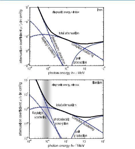
2.3 |
Photon–Matter Interaction |
|
Fig. . . Mass attenuation coe cient, μ ρ, versus incident photon energy for iron (top) and titanium (bottom). For the diagnostic energy window of CT, E = [ keV– keV], photoelectric absorption is dominant in the low-energy part and Compton scattering is dominant in the high-energy part of the diagnostic window (compiled with data from the web database XCOM [Berger et al. ])
coe cient is a function of the spatial coordinates and photon energy. However, on the other hand, the spatial distribution of the attenuation coe cient μ is the main focus of diagnostic interest. The gray-value di erences in CT images represent distinct material composites and densities of the organs. The normal CT image shall be seen as standard, as radiologists learn, and any variation of that standard is potentially pathologic.
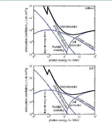
2 Fundamentals of X-ray Physics
Fig. . . Mass attenuation coe cient, μ ρ, versus incident photon energy for platinum (top) and gold (bottom). For the diagnostic energy window of CT, E = [ keV– keV], photoelectric absorption is dominant (compiled with data from the web database XCOM [Berger et al. ])

2.3 |
Photon–Matter Interaction |
|
Fig. . . Mass attenuation coe cient, μ ρ, versus incident photon energy for amalgam (top:% Sn, Z = ; % Hg, Z = ; % Ag, Z = ) and for compact bone (bottom: % H, Z = ; % C, Z = ; % N, Z = ; % O, Z = ; % P, Z = ; % Ca, Z = ). For the diagnostic energy window of CT, E = [ keV– keV], photoelectric absorption is dominant for amalgam and Compton scattering is dominant for bone (compiled with data from the web database XCOM [Berger et al. ])

2 Fundamentals of X-ray Physics
2.4
Problems with Lambert–Beer’s Law
From a mathematical point of view, the complicated dependency of the attenuation coe cient on the property of the penetrated material means that the di erential equation ( . ) cannot be fully integrated as shown in ( . ). In the case of spatially
varying attenuation, μ(η |
) |
, the solution for the intensity after a running length, s, is |
|||
given by |
|
s |
|
|
|
|
|
I(s) = I( )e |
|
|
|
|
|
− ∫ μ(η)dη |
, |
( . ) |
|
|
|
|
|||
summing up the unknown coe cients along the X-ray beam within the exponent. A second point to mention is the energy dependence of the attenuation values, which is not modeled by ( . ). Hence, ( . ) must be extended to
I(s) = |
Emax |
s |
μ(E,η)dη |
|
∫ |
− ∫ |
|
||
I (E)e |
dE . |
( . ) |
The di erence between ( . ) and ( . ) is the origin of what is called the beamhardening artifact. However, in practice, only ( . ) is used. Therefore, this is the basic model that will be used throughout this book. As one is especially interested in the spatial variation of the attenuation, i.e., in the inversion of the integral operation in ( . ), the projection integral
( ) = − |
|
|
|
( |
s |
) = |
|
|
|
I |
|
|
|
p s |
ln |
|
I |
( ) |
||
s |
|
∫ μ(η)dη |
( . ) |
is defined for convenience. It is essentially the negative logarithm of the ratio of the incoming and outgoing number of photons.
In the technical realization of CT, one is restricted to a certain discretization of the reconstructed images. When an X-ray beam runs through the continuous matter, such a partitioning of the penetrated material cannot be physically measured. Nevertheless, one can model the matter to be discrete and calculate the total attenuation for this case. If the attenuation coe cient varies discontinuously, as schematically indicated in Fig. . , the intensity reduction while running through the tissue can be estimated without solving a di erential equation.
|
In this model, the attenuation |
|
|
|
|
|
|
|
|||
|
|
Ii + |
|
Ii μi + Ii |
η Ii |
|
μi + η |
|
( . ) |
||
of the intensity Ii |
resulting in the intensity I |
when running through the tissue, |
|||||||||
|
= |
− |
=i +( |
|
− |
|
|
) |
|
||
i , of thickness |
η, and attenuation coe cient, μi + , can be obtained. Conse- |
||||||||||
quently, the total attenuation is a series of products |
|
|
|
|
|||||||
+ |
In = I ( − μ |
η)( − μ |
η)( − μ |
η) ( − μi |
η) ( − μn η) . |
( . ) |
|||||
|
|||||||||||
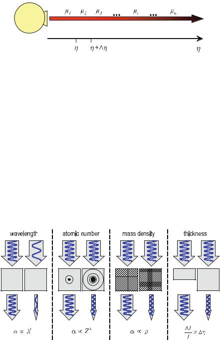
|
|
|
|
2.4 Problems with Lambert–Beer’s Law |
|
||||
|
|
|
|
|
|
|
|
|
|
|
|
|
|
|
|
|
|
|
|
Fig. . . Attenuation of an X-ray beam while running through a tissue that is modeled by a sequence of discontinuous partitions
If the discretization of the tissue is very fine, i.e., η is chosen to be small, the factor terms in parentheses can be interpreted as the Taylor expansion of the exponential function. With
for small δ, the approximation |
e−δ − δ |
|
|
|
|
|
|
|
( . ) |
|||||
In |
|
I e−μ η e−μ |
η e−μ η e−μi |
|
η |
|
|
e−μn η |
( . ) |
|||||
can be obtained. By |
taking the limit δ |
the exact equation |
|
|||||||||||
|
|
|
|
μi η |
|
|
|
|
|
|
|
|
||
|
|
|
In = I e |
n |
I e− |
∫ μ |
( |
η |
) |
dη |
|
( . ) |
||
|
|
|
i = |
|
|
|||||||||
|
|
|
|
− |
|
|
|
|
|
|
|
|||
can be obtained. This view on the modeling of X-ray attenuation is closely related to a statistical view of photon number reduction by photon–matter interaction that will be introduced at the end of this chapter. To summarize the facts above, it can be said that the attenuation of X-ray through matter is well understood and thus,
Fig. . . Causes of attenuation: Wavelength of the incident beam, atomic number, mass density, and thickness of the medium (after Laubenberger and Laubenberger [ ])
|
2 Fundamentals of X-ray Physics |
|
|
|
|
the gray values of the CT images are a direct physical representation of the material |
|||
|
properties. This is clearly an advantage in comparison to MRI, where the gray values |
|||
|
can be tuned by various parameters of complicated scanning protocols such that the |
|||
|
direct relation to physical properties is lost. In CT, high values of the attenuation |
|||
|
coe cient, μ, are due to a high density or high atomic number of the medium. |
|||
|
In Fig. . , the relationship between the attenuation and the wavelength of the |
|||
|
incident beam, as well as the atomic number, density, and thickness of the material, |
|||
|
is schematically summarized. |
|
|
|
|
In Chaps. – the reconstruction of non-superimposed object slices will be |
|||
|
derived and discussed in detail. Within the calculation of the spatial distribution |
|||
|
of the attenuation coe cient, μ |
x, y |
) |
, the projection modeled by ( . ) and ( . ) |
|
must be reversed in some sense.( |
|
|
|
2.5
X-ray Detection
Since the main interaction principles between X-ray photons and matter have been explained in the section above, no new e ects have to be introduced to explain the interaction between X-ray radiation and the detector material. Consequently, X-ray quanta are not measured directly, but are detected via their interaction products (for example, emitted photoelectrons). The overall detection e ciency is primarily determined by the geometric e ciency (also called the fill factor) and the quantum e ciency (also called the capture e ciency) (Cunningham ). The geometric e ciency refers to the X-ray sensitive area of the detector as a fraction of the total exposed area, and the quantum e ciency refers to the fraction of incident quanta that are absorbed and contribute to the signal. The overall detection e ciency is the product of the geometric and the quantum e ciency.
2.5.1
Gas Detectors
X-ray radiation is able to ionize gases. This fact was discovered very early in the last century and led to the development of the well-known Geiger–Müller counter. In the first tomographic experiments carried out by Cormack and Hounsfield, the Geiger– Müller counter was used as a detector in pencil-beam geometry. In the early days of clinical CT, gas-based detector arrays were also manufactured for what are known as third-generation scanners in fan-beam geometry. Even today, some scanners using high-pressure xenon are in use. The photoelectric interaction,
hν + Xe Xe+ + e− , ( . )

2.5 X-ray Detection |
|
describes the first part of the detection process chain. Xenon ions and electrons are attracted by high voltage to a cathode and an anode respectively. A series of alternating cathode and anode pairs forms the detector array. Figure . schematically shows the reaction chain starting with the photoelectric ionization to the recombination of the free charged particles at the electrode surfaces. The current produced by recombination is a measure of the X-ray intensity entering the detector.
A weak quantum e ciency (a low probability for the photoelectric absorption) can be compensated for by a high pressure and by tall ionization chambers. Another advantage of tall chambers is improved directional selectivity of the detector element. Since the ionization probability is proportional to the travel length of X-ray quanta inside an element (one cathode–anode block), detection of X-ray quanta with an oblique entrance will be suppressed. In this way, a tall detector element has a built-in collimation. However, septa between detector elements are insensitive regions that will decrease the geometric e ciency of the detector.
Fig. . . Schematic cut-out of two adjacent ionizing chambers of a xenon high-pressure detector array. Since the chambers are communicating, all detector elements have the same Xe pressure and, therefore, the same sensitivity
|
2 Fundamentals of X-ray Physics |
||||||||||
|
2.5.2 |
|
|
|
|
|
|
|
|
|
|
|
Solid-State Scintillator Detectors |
||||||||||
|
Today, almost all modern CT systems are equipped with scintillator detectors. Such |
||||||||||
|
a detector essentially consists of two main components: A scintillator medium and |
||||||||||
|
a photon detector. In a first step, the short-wave X-ray radiation entering the detec- |
||||||||||
|
tor is converted into long-wave radiation (light) inside the scintillation media. Typ- |
||||||||||
|
ical scintillator materials used are cesium iodide (CsI), bismuth germanate (BGO) |
||||||||||
|
or cadmium tungstate (CdWO ). The choice of material is critical and depends on |
||||||||||
|
the desired quantum e ciency for the conversion from X-ray to light and on the |
||||||||||
|
time constant for the conversion process, which determines the afterglow of the de- |
||||||||||
|
tector. |
||||||||||
|
For a very fast fluorescence decay, i.e., a very small time constant, as required |
||||||||||
|
by modern sub-second scanners, ceramic materials made of rare earth oxides like |
||||||||||
|
gadolinium oxysulphide (Gd O S) are used (Kalender ). To assess the quality |
||||||||||
|
of a detector material with respect to the desired behavior of high quantum e - |
||||||||||
|
ciency, the mass attenuation coe cient must be known. In Fig. . it can be seen |
||||||||||
|
|
|
|
|
|
|
|
|
|
|
|
|
|
|
|
|
|
|
|
|
|
|
|
|
|
|
|
|
|
|
|
|
|
|
|
|
|
|
|
|
|
|
|
|
|
|
|
Fig. . . Mass attenuation coe cient for the main photon–matter interaction principles in detector materials. Photoelectric absorption is more than one magnitude higher than scattering processes in xenon and the Gd O S-ceramic. Due to the fact that, inside the relevant diagnostic energy window, the mass attenuation coe cient due to photoelectric absorption for Gd O S is higher than for xenon, the quantum e ciency of the ceramic detector material is superior. This holds especially true, since the density of the solid-state detector material is obviously higher than the density of xenon
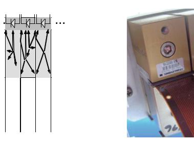
2.5 X-ray Detection |
|
that the Gd O S ceramic has a higher probability of energy conversion via photoelectric absorption than xenon. Due to the fact that the mass density ρ of the gas xenon is three magnitudes smaller than the mass density of the solid-state detector material, the e ective absorption of quanta inside the solid-state detector, and therefore its quantum e ciency, is significantly higher. This can be only partially compensated by long Xe chambers and a high gas pressure.
In Fig. . the components of a scintillator detector unit are shown schematically. On the right-hand side of Fig. . a detector unit of the Philips Tomoscan EG is shown. One unit consists of detector elements. X-rays that have been scattered may undergo deflection through a small angle and finally reach the detector. This is an undesired detection because it reduces the image contrast. To suppress the measurement of scattered X-ray quanta, collimator lamella are attached to each element. Such an anti-scatter collimator grid is directed toward the X-ray focus to filter out photons not traveling in the line of sight between X-ray source and detector. Without an anti-scatter grid, the image quality would be significantly reduced.
However, there is an obvious disadvantage of the anti-scatter grid. To block an oblique entrance of scattered X-ray photons e ectively, a minimum lamella thickness of . mm is required. In practice, the detector elements have a total geometric e ciency of about – % (Kalender ). This decreased fill factor leads to an undesired reduction in spatial detector resolution.
Fig. . . Schematic drawing and photograph of a detector unit. Single detection channels are separated by thin anti-scatter lamella. The scintillator medium converts the X-ray quanta to light, which subsequently is detected by a photodiode mounted on the crystal
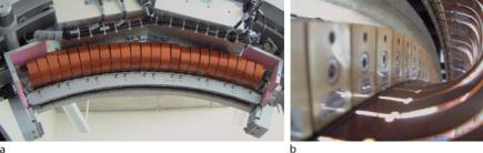
|
2 Fundamentals of X-ray Physics |
Fig. . a–b. Uncovered detector array of the compact Philips Tomoscan EG scanner. a Ribbon cable connections of detector units, each consisting of channels, above the antiscatter grid. b Arrangement of the detector units in a circle segment
On the rotating sampling unit, the series of detector elements is arranged in a circle segment with the X-ray source at its center. In Fig. . a detector array with units, each with channels, is shown.
2.5.3
Solid-State Flat-Panel Detectors
Crystaland ceramic-based solid-state detectors described in the previous section can be extended to multi-row or multi-slice detector systems. The key feature of such multi-row arrays is a maximum e ective X-ray-sensitive area. This feature is quantified by the fill factor, which is explained below. Xenon high-pressure gas detector array systems cannot be easily extended to flat area detector systems. Therefore, all modern multi-slice CT systems are based on solid-state scintillation detectors.
In Fig. . , a cone-beam detector system is drawn schematically. In contrast to detector systems in technical CT systems, for example, in micro-CT (where flatpanel detectors are employed) almost all clinical CT systems are equipped with cylindrical detector units. As illustrated in Fig. . the multi-array system forms a cylinder barrel with the X-ray source as its center. If the number of rows of such multi-slice detector systems is chosen to be very high, the orientation of the respective X-ray fan inside the cone beam, relative to the axial slice, becomes significant, and the requirements of image reconstruction increase. However, modern CT systems are equipped with cone-beam sampling units due to improved spatial resolution and faster image acquisition. Image reconstruction in cone-beam systems will be discussed in Chap. .
In Fig. . , di erent technical configurations of multi-slice detector systems used in Siemens (left) and General Electric (right) multi-slice CT (MSCT) systems are shown. T he Siemens detector is a UFCTM adaptive array detector. This detector unit is partitioned into either slices measuring . mm thick or slices measuring . mm thick. The flexibility is achieved by the interconnection of pairs of
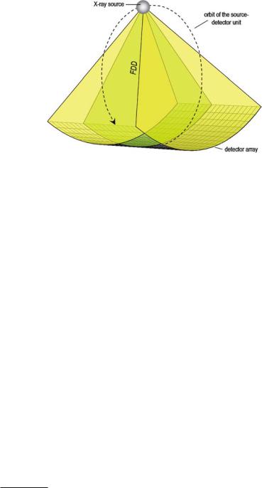
2.5 X-ray Detection |
|
Fig. . . Cone-beam illumination of a cylindrical detector system. The multi-array system forms a cylinder barrel with the X-ray focus as its center. The source-detector sampling unit, with diameter FDD (Focus-Detector-Distance), is rotating on a circle (dashed line) with the iso-center inside the field of measurement
detector segments. The General Electric detector type, shown here, has spatially equidistant rows of detector elements. However, an electronic combination of the rows results in flexible slice thickness as well.
Without reconstruction mathematics that are adapted to the cone-beam situation, image artifacts arise for the higher X-ray fan angulations, even in a -row detector system. This leads to clinically unacceptable image quality. In any case, the reconstruction algorithms used for the cone-beam geometry need to be revised for practical implementation. Therefore, it is a consequent step to leave the multirow detector arrays and move in the direction of real flat-panel detector systems. These systems have recently become commercially available. However, they were not originally designed for use in CT systems, but rather to compete with established radiography systems using film cassettes, computed radiography cassettes, and image intensifiers.
In Fig. . , the typical composition of such a digital flat-panel X-ray detector is shown. In Fig. . a, the key aspect of the construction is illustrated. Each sensor element consists of a photodiode and a thin-film transistor (TFT). Both are made of amorphous silicon on a single glass substrate. The pixel matrix is coated with an X-ray-sensitive layer. Multi-chip modules are used as read-out electronics at the edge of the detector field. The X-ray-sensitive coating is a cesium iodide layer used, for example, in General Electric CT systems. The basis is the single glass substrate with a silicon matrix of , , sensors, each μm in size. The monolithic structuring is done with thin-film technology such that a composition of a set of medium-sized sub-panels, which have undesired dead zones at the in-
Pixel is an acronym composed of picture and element, using the abbreviation ‘pix’ for picture.
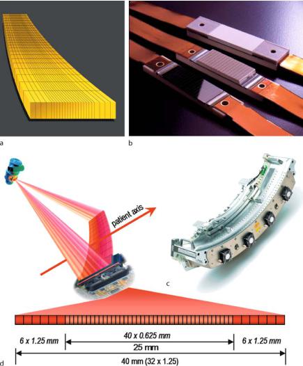
|
2 Fundamentals of X-ray Physics |
Fig. . a–d. Detector parts used for multi-slice detector technology – courtesy of Siemens Medical Solutions (a, c), General Electric Medical Systems (b), and Philips Medical Systems (d)
terfaces, potentially producing imaging artifacts, is not required. The final coating with cesium iodide (CsI) is the required scintillator layer of the detector. The CsI layer is applied directly onto the pixel matrix by a physical deposition process.
The production technique is known from semiconductor production. Physical and chemical processing steps, i.e., the combination of photolithography and further etching phases, are applied to produce these finely structured detector

2.5 X-ray Detection |
|
Fig. . . Left: Composition of a digital flat-panel X-ray detector. Right: Schematic illustration of the signal conversion chain inside the detector (courtesy of General Electric Medical Systems: Brunst [ ])
elements. This leads to an X-ray-sensitive detector field with a desired high fill factor,
f = |
X-ray sensitive area of the detector |
, |
( . ) |
total area of the detector |
that cannot be produced by the simple combination of the detector types described in Sects. . . and . . .
In Fig. . , the signal processing flow inside the X-ray detector is illustrated schematically. X-ray quanta entering the detector are converted into visible light in the upper CsI scintillator layer. The light photons are guided to the photodiodes of the next processing layer. The photons are absorbed, thereby producing an electric charge in the photodiodes that is proportional to the intensity of the X-ray radiation. During detector exposure, the electric charge is integrated and stored in the detection element, which acts as capacitor. The actual read-out process is initialized by the thin-film transistor, which switches the charge to the read-out electronics via the data link. There, an amplification and the analog-to-digital conversion is performed on the same chip, resulting in fast operation with low noise. Figure . illustrates that the flat-panel detector system has a very high fill factor. In Fig. . , a preassembly, raw detector with ribbon cable data links as well as a post-assembly, digital flat-panel detector that is ready for application, are shown. Its , , pixels are integrated onto an active cm area.
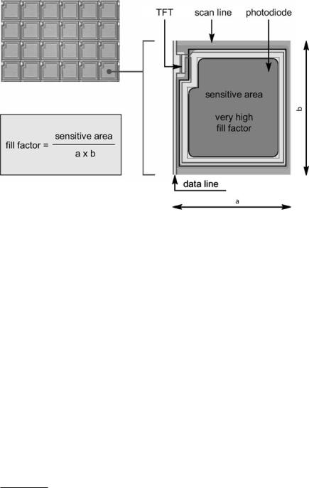
|
2 Fundamentals of X-ray Physics |
Fig. . . Schematic illustration of the flat detector field and a single detector element of the field. The quality of the detector is influenced by the size of the X-ray-sensitive detector area. Insensitive areas such as splices of space for electronics must be minimized. The measure of this geometric detector quality is the fill factor, i.e., the ratio between the X-ray-sensitive area and the total area of the sensor (courtesy of General Electric Medical Systems: Brunst [ ])
A highly desired system property of the digital scintillation detector system is the linear dynamics over a wide range of illumination. In this way, highand lowdose applications have the same contrast information, i.e., excellent contrast resolution. Figure . shows the characteristic response diagrams of the signal dynamics of an analog film system and a digital scintillator system respectively . Film systems are capable of imaging objects with high contrast within a very narrow exposure range only. If the object is overor underexposed, the contrast of the image can easily be too low. Due to the linear characteristic response curve of the digital system, it is robust against overand underexposure. However, within the range of low-contrast imaging, flat-panel systems do not achieve the quality of dedicated CT detector systems described in the sections above (Kalender ).
In addition to the linear characteristic diagrams of the detector dynamics, another important advantage of the flat-panel detector is its excellent spatial resolution. To optimize the spatial resolution, cesium iodide is evaporated onto the matrix so that direct contact between the scintillation material and the carrying photodiode matrix is established. This manufacturing step is designed so that cesium io-
Flat-panel detector systems were developed for use in simple radiography systems to replace film systems or computed radiography cassettes.
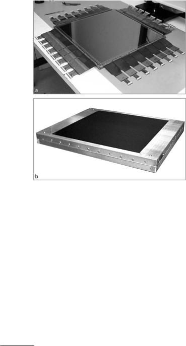
2.5 X-ray Detection |
|
Fig. . . Realization of a cm cm flat-panel detector integrating , , pixels. a Pre-assembly panel with ribbon cable for read-out electronics. b Complete flat-panel system ready for use (courtesy of General Electric Medical Systems: Brunst [ ])
dide grows anisotropically, forming needles on the matrix. In Fig. . , the needle structure of CsI is demonstrated in an electron microscope picture. If X-ray quanta are converted into visible light inside the CsI structure , the emerging photons are, in all likelihood, traveling along the needles, because they act as a fiber-optical cable. In this way photons are guided directly onto the photodiode or in the opposite direction. The photons that are traveling in the opposite direction face a mirror on the top side of the CsI layer that ensures that eventually almost all photons find their way to the photodiode. This light guidance e ect of the CsI fiber structure is the reason for the high quantum e ciency of the digital flat-panel detectors. The X-ray-sensitive CsI coating can be made very thick to obtain a high quantum e - ciency and to also suppress broad photon scattering, which would reduce the spatial resolution. The scintillation light is bundled by the CsI fibers onto a small point on the photodiode matrix. However, an isotropic CsI layer must always find a compromise between high quantum e ciency and high spatial resolution.
Typically, a cloud of about , optical photons, each with energy of approximately eV, is generated by an X-ray quantum of several tens of keV.

|
2 Fundamentals of X-ray Physics |
||||||||
|
|
|
|
|
|
|
|
|
|
|
|
|
|
|
|
|
|
|
|
|
|
|
|
|
|
|
|
|
|
|
|
|
|
|
|
|
|
|
|
|
|
|
|
|
|
|
|
|
|
|
|
|
|
|
|
|
|
|
|
Fig. . . Comparison of dynamic characteristics between a film detector system (left) and a digital scintillation detector (right). Besides a desired linearity of the digital detector, the dynamic range of the scintillation detector of – , : (compared with – : of the film detector) is also superior (Brunst )
Fig. . . The cesium iodide scintillation layer of a flat-panel detector element (picture taken with an electron microscope, courtesy of General Electric Medical Systems: Brunst [ ])

2.6 X-ray Photon Statistics |
|
Fig. . . A digital flat-panel detector mounted on an experimental rotating C-arm device for testing cone-beam reconstruction algorithms (courtesy of General Electric Medical Systems)
In Fig. . a digital flat-panel detector mounted on an experimental C-arm device is shown. The device can be rotated and, therefore, used to demonstrate the feasibility of cone-beam tomographic imaging. C-arm-based tomographic devices are relatively small and inexpensive compared with complete CT systems. On the other hand, they exhibit mechanical instabilities with reduced spatial resolution. However, there is a demand for interventional three-dimensional imaging modalities. This is because surgeons would like to add intra-operative three-dimensional CT information to endoscopic or ultrasound imaging in minimally invasive operations, but typically there is not enough space for a normal CT system in an operating room (Härer et al. ). Compared with clinical CT systems, a disadvantage of the flat-panel C-arm-based apparatus is the small diameter ( cm or less) of the imaging field (Härer ).
2.6
X-ray Photon Statistics
X-ray radiation consists of X-ray quanta with specific statistical properties that must be considered in many fields of X-ray signal processing applications. It will be shown later in this book that particular reconstruction methods can be applied in CT that are based on the statistical nature of X-ray quanta. Furthermore, the evaluation of image quality is based upon the physically correct model of noise statistics.
The next sections will focus on the statistical properties of the X-ray source and on those of the X-ray detector. As with many stochastic processes, the statistics of X-ray generation and interaction with matter can be understood in the limit
|
2 Fundamentals of X-ray Physics |
|
|
|
|
|
||||||
|
of processes with binomial probability densities. Additionally, Lambert–Beer’s law |
|||||||||||
|
of photon absorption will be discussed in terms of photon statistics and the most |
|||||||||||
|
important moments of Poisson-distributed random variables will be addressed. In |
|||||||||||
|
the final sections the central-limit theorem and non-Poisson measurement will be |
|||||||||||
|
discussed. |
|
|
|
|
|
||||||
|
2.6.1 |
|
|
|
|
|
|
|
|
|
|
|
|
Statistical Properties of the X-ray Source |
|
|
|
|
|
||||||
|
Statistical reconstruction techniques like the maximum likelihood expectation max- |
|||||||||||
|
imization (MLEM) approach, which will be introduced in |
|
Sect. . , are based on |
|||||||||
|
the exact knowledge of quantum number statistics. The |
probability density func- |
||||||||||
|
|
|
|
|
|
|||||||
|
tion is explicitly incorporated in the method. Therefore, a mathematical model of |
|||||||||||
|
the physical nature of X-ray quanta must first be found. |
|
|
|
|
|
||||||
|
To derive the statistical photon model, the section begins with a discussion of |
|||||||||||
|
the X-ray quanta generation statistics inside the focus area on the X-ray tube anode. |
|||||||||||
|
As mentioned at the beginning of this chapter, the lattice atoms of the anode ma- |
|||||||||||
|
terial are bombarded with fast electrons that are accelerated during their transit |
|||||||||||
|
from the cathode to the anode. In Fig. . , this situation is illustrated. Let N elec- |
|||||||||||
|
trons arrive at the active focus volume in the time window |
[ , T] and, let each of |
||||||||||
|
|
|
|
|
|
|
|
|
|
|
|
|
|
|
|
|
|
|
|
|
|
|
|
|
|
|
|
|
|
|
|
|
|
|
|
|
|
|
|
|
|
|
|
|
|
|
|
|
|
|
|
|
|
|
|
|
|
|
|
|
|
|
|
|
|
|
|
|
|
|
|
|
|
|
|
|
|
|
|
|
|
|
|
|
|
|
|
|
|
|
|
|
|
|
|
|
|
|
|
|
|
|
|
|
|
|
|
|
|
|
|
|
|
|
|
|
|
|
|
|
|
|
|
|
|
|
|
|
|
Fig. . . X-ray quanta generation as a statistical counting process

2.6 X-ray Photon Statistics |
|
the N electrons have a probability, p (with p ), of interacting in the same time interval with one of the target atoms in such a way that an X-ray quantum emerges.
It is also assumed that each collision process between fast electrons and target atoms in the lattice is statistically independent of all other collisions inside the focus volume. Then, the probability, P, that the random variable, N, i.e., the number of emerging X-ray quanta, is assigned exactly to the number n is
P (N = n) = n pn ( − p)N−n . |
( . ) |
N |
|
This means that the number of X-ray quanta, N, is a binomially distributed random variable with N out of , . . . N . ( . ) is the well-known Bernoulli distribution, which measures the probability that n successful outcomes occur in a sequence of N independent trials. The term
N |
|
N! |
|
n |
= |
|
( . ) |
n!(N − n)! |
is the binomial coe cient and can be visualized by Pascal’s triangle , illustrated in Fig. . . The term is sometimes also read as “N chooses n”.
It is well known that the statistics of independent coin-throwing experiments can be modeled by the Bernoulli distribution. The probability of heads and tails is p = . . The Bernoulli distribution is the simplest discrete distribution, and it is a building block for other, more complicated discrete distributions.
Fig. . . Pascal’s triangle
Actually, years before Pascal studied the number triangle, the Chinese mathematician Yang Hui described the triangle first. Therefore, in China it is known as Yang Hui’s triangle.

|
2 Fundamentals of X-ray Physics |
Obviously, the generation of X-ray quanta can be statistically interpreted as a counting process. ( . ) is a normalized discrete probability distribution, where
N |
|
(N = |
|
N |
|
N |
|
|
( |
|
− |
|
) |
|
= ( |
|
+ ( |
|
− |
|
)) |
|
= |
|
|
|
P |
n |
) = |
pn |
|
p |
N−n |
p |
|
p |
N |
. |
( . ) |
||||||||||||
n = |
|
|
|
n = |
|
n |
|
|
|
|
|
|
|
|
|
|
|
|
|
|
|
|
|
|
|
However, a realistic magnitude of the number of fast electrons arriving at the focus volume in the time interval, [ , T], can be approximated via the anode current. Let I = mA, a typical current used for medical CT. Then, the number of electrons arriving in ms is
N = T |
I |
= − s ċ |
. A |
. |
( . ) |
e |
. ċ − As |
On the other hand, the probability, p, of a successful collision is very small. It has been mentioned above that this small probability, or e ciency, of the X-ray quanta creation process is the reason for the considerable heat problem of X-ray tubes.
In practice, the number of arriving electrons and the probability of successful collision can be expressed in the limits N and p respectively. However, since an X-ray tube produces X-ray quanta, there must be a positive number of photons in the limit of Np n , where E[N] = n is the expectation value of the number of X-ray quanta. This leads to a certain limit of the Bernoulli distribution that will be derived below.
Assume that
|
|
|
|
|
|
|
|
|
|
|
|
|
|
|
|
|
|
|
|
Np |
|
n |
|
|
|
|
|
|
|
|
|
|
|
|
|
|
|
|
|
|
|
|||||||||
and substitute ( . ) into ( . ), resulting=in |
|
|
|
|
|
|
|
|
|
|
|
|
|
|
|
|
|
|
|
|||||||||||||||||||||||||||||||
|
(N = |
|
|
N |
|
|
|
( |
|
− |
) |
|
|
|
|
|
|
|
|
|
N |
|
|
n |
|
n |
|
|
|
− |
n |
|
N−n |
|
||||||||||||||||
|
|
) = n |
pn |
|
N |
−n |
n= n |
|
|
N |
n |
|
|
|
|
|
|
|
|
|||||||||||||||||||||||||||||||
P |
|
n |
|
|
|
|
|
|
|
|
|
p |
|
|
|
|
|
|
|
|
|
|
|
|
|
|
|
|
|
|
|
|
|
|
|
|
|
|
|
|
|
|
|
|||||||
|
|
|
|
|
|
|
|
|
|
|
|
|
|
|
|
|
|
|
|
|
|
|
|
|
|
|
|
|
|
|
|
|
|
N |
|
|
|
|
|
|
|
|
N |
|
|
|
|
|
||
|
|
|
= |
|
|
|
N! |
|
|
|
|
|
n |
− |
|
n |
|
|
|
|
− |
|
|
|
|
|
|
|
|
|
|
|
|
|
|
|||||||||||||||
|
|
|
n!(N − n)! |
|
N |
|
|
N |
|
|
n |
|
|
|
|
|
|
|
|
n N |
|
|
||||||||||||||||||||||||||||
|
|
|
= ( − ) ( − ( − )) |
|
|
|
|
|
|
|
|
|
|
N |
n |
|
|
|||||||||||||||||||||||||||||||||
|
|
|
|
N N |
|
|
|
|
|
|
N |
|
|
|
|
|
|
n |
|
|
|
|
|
|
|
|
|
|
|
|
|
|
|
N |
|
|
||||||||||||||
|
|
|
|
|
|
|
|
|
|
|
|
|
|
n! |
|
|
|
|
|
|
|
|
|
|
|
|
|
|
|
|
N |
|
n |
|
− |
n |
|
|
||||||||||||
|
|
|
|
|
( |
|
|
− ) ( |
|
|
|
|
− ( |
|
|
− )) |
|
|
|
|
|
N− |
|
|
|
|
|
|||||||||||||||||||||||
|
|
|
|
|
|
|
|
|
|
|
|
|
|
|
|
|
|
|
|
|
|
|||||||||||||||||||||||||||||
|
|
|
|
N |
N |
N |
|
|
n |
|
|
|
|
|
|
n |
|
|
|
|
|
|
|
|
|
|||||||||||||||||||||||||
|
|
|
= |
|
|
|
|
|
|
|
|
|
|
|
|
|
|
|
|
|
|
− |
|
|
|
|
|
|
|
|
|
|||||||||||||||||||
|
|
|
|
|
|
|
|
|
|
|
|
n |
|
|
|
|
|
|
|
|
n |
|
|
|
|
|
|
|
|
|
|
|
|
|
|
|
|
|
|
|
|
|||||||||
|
|
|
|
|
|
|
|
|
|
|
|
|
|
N |
|
|
− |
|
|
|
|
|
|
|
|
|
|
|
|
|
|
|
N |
|
|
|
|
|
|
|
|
|
||||||||
|
|
|
|
|
|
|
|
|
n! |
|
|
|
|
|
|
|
|
|
|
|
|
|
|
|
|
|
|
|
|
|
|
|
|
|
|
|
|
|
|
|
|
|
||||||||
|
|
|
|
|
|
|
|
|
|
|
|
|
|
|
|
|
|
|
|
|
|
|
|
|
|
|
( − |
|
|
) |
|
|
|
|
|
|
n |
|
|
. |
||||||||||
|
|
|
|
|
|
|
|
|
|
|
|
|
|
|
|
|
|
|
|
|
|
|
|
|
|
|
|
|
|
|
|
|
|
|
|
|
|
|
|
|||||||||||
|
|
|
|
|
|
|
|
|
|
|
|
|
|
|
|
|
|
|
|
|
|
|
|
|
|
|
|
|
|
|
|
|
|
|
|
|
|
|
|
|||||||||||
|
|
|
|
|
|
|
|
|
|
− |
|
|
|
|
ċ ċ ċ ċ |
|
− |
|
|
|
|
! |
|
|
|
|
|
|||||||||||||||||||||||
|
|
|
|
|
|
|
|
Nn |
|
|
|
|
|
|
|
|
|
|
|
|
|
|
|
|
|
|
|
|
|
n |
|
|
|
|
|
|
|
|
|
|
|
|
|
N |
||||||
|
|
|
= |
|
|
|
|
|
|
|
|
|
|
|
|
|
|
|
n |
− |
N |
|
|
|
|
|
|
|
|
|
|
|
" − |
|
|
|
|
|||||||||||||
|
|
|
|
|
|
|
|
|
|
|
|
|
|
|
|
|
|
|
|
|
|
|
|
|
|
|
|
|
|
|
|
|
|
|
|
|
# |
|
|
|
|
|
|
|
||||||
|
|
|
|
n! |
|
|
|
|
|
|
|
Nn |
|
|
|
|
|
|
|
|
|
|
|
|
|
|
|
|
|
|
|
|
|
|
|
|
|
" |
|
|
|
N |
|
|
||||||
( . )
( . )

|
|
|
|
|
|
|
|
|
|
|
|
|
|
|
|
|
|
|
|
|
|
|
|
|
|
|
|
|
|
|
|
|
|
|
|
|
|
|
|
|
|
|
|
|
|
|
|
|
|
2.6 |
|
|
X-ray Photon Statistics |
|
||||||||||||||
In the limit N |
|
|
|
, the second term in the last row of ( . ) is |
( |
n |
) |
n . T he last |
|
|||||||||||||||||||||||||||||||||||||||||||||||||||||||||||
term is given by |
|
|
|
|
|
|
|
|
|
|
|
|
|
|
|
|
|
|
n |
N |
|
|
|
|
|
|
|
|
|
|
|
|
|
|
|
|
|
|
|
|
|
|
|
|
|
|
|
|
|
|
|
|
||||||||||||||||
|
|
|
|
|
|
|
|
|
|
|
|
|
|
|
|
|
|
|
|
|
|
|
|
|
|
|
|
|
|
|
|
n |
|
|
|
|
|
|
|
|
|
|
|
|
|
|
|
|
|
|
|
|
|
|
|
|
|
|
||||||||||
|
|
|
|
|
|
|
|
|
|
|
|
|
|
|
lim |
|
|
|
|
|
|
|
|
|
|
|
|
= e |
− |
|
|
|
|
|
, |
|
|
|
|
|
|
|
|
|
|
|
|
|
|
|
|
|
|
|
|
|
( . ) |
|
||||||||||
|
|
|
|
|
|
|
|
|
|
|
|
|
|
|
|
|
|
|
|
|
|
|
|
|
|
|
|
|
|
|
|
|
|
|
|
|
|
|
|
|
|
|
|
|
|
|
|
|
|
|
|
|
|
|||||||||||||||
|
|
|
|
|
|
|
|
|
|
|
|
|
|
N − N |
|
|
|
|
|
|
|
|
|
|
|
|
|
|
|
|
|
|
|
|
|
|
|
|
|
|
|
|
||||||||||||||||||||||||||
which can easily be shown, because |
|
|
|
|
|
|
|
|
|
|
|
|
|
|
|
|
|
|
|
|
|
|
|
|
|
|
|
|
|
|
|
|
|
|
|
|
|
|
|
|
|
|
|
|
|
|
|
|||||||||||||||||||||
|
|
|
|
|
N |
|
|
− |
n |
|
N |
|
= N − |
|
n |
|
N |
|
|
|
|
|
|
|
|
|
( . ) |
|
||||||||||||||||||||||||||||||||||||||||
|
|
|
|
|
|
N |
|
|
|
|
N |
|
|
|
|
|
|
|
|
|
|
|
|
|||||||||||||||||||||||||||||||||||||||||||||
|
|
|
|
|
|
lim |
|
|
|
|
|
|
|
|
|
|
|
|
|
|
lim |
|
|
|
exp |
ln |
|
|
|
|
|
|
|
|
|
|
n |
|
|
|
|
|
|
|
|
|
|
|
|
|
|
|
||||||||||||||||
|
|
|
|
|
|
|
|
|
|
|
|
|
|
|
|
|
|
|
|
= N exp N ln − |
|
|
. |
|
|
|
|
|
|
|
|
|||||||||||||||||||||||||||||||||||||
|
|
|
|
|
|
|
|
|
|
|
|
|
|
|
|
|
|
|
|
|
|
N |
|
|
|
|
|
|
|
|
|
|||||||||||||||||||||||||||||||||||||
|
|
|
|
|
|
|
|
|
|
|
|
|
|
|
|
|
|
|
|
|
|
|
lim |
|
|
|
|
|
|
|
|
|
|
|
|
|
|
|
|
|
|
|
|
|
|
|
|
|
|
|
|
|
|
|
|
|
|
|
|
|
|
|
|
|||||
With the expansion of the logarithm, |
(% )i |
x |
|
|
for |
|
|
|
|
|
|
|
x |
|
|
|
|
|
|
, |
|
|
|
|
|
|
|
|
|
( . ) |
|
|||||||||||||||||||||||||||||||||||||
|
|
|
|
|
|
|
|
ln |
x |
|
|
|
|
|
|
|
i = |
|
|
i |
|
|
|
|
|
|
|
|
|
|
|
|
|
|
|
|
|
|
|
|
|
|
|
|||||||||||||||||||||||||
|
|
|
|
|
|
|
|
|
( $ |
|
|
|
|
|
|
|
|
|
|
|
|
|
|
|
|
|
i |
|
|
|
|
|
|
− |
|
|
< |
|
|
|
< + |
|
|
|
|
|
|
|
|
|
|
|
|
|
|
|||||||||||||
one obtains |
|
|
|
|
|
) = − |
|
|
|
|
|
|
|
|
|
|
|
|
|
|
|
|
|
|
|
|
|
|
|
|
|
|
|
|
|
|
|
|
|
|
|
|||||||||||||||||||||||||||
|
|
|
|
|
|
|
|
|
|
|
|
|
|
|
|
|
|
|
|
|
|
|
|
|
|
|
|
|
|
|
|
|
|
|
|
|
|
|
|
|
|
|
|
|
|
|
|
|
|
|
|
|
|
|
|
|
|
|
|
|
|
|
|
|||||
N |
|
|
|
n |
|
N |
= N |
|
|
|
|
|
|
|
|
|
|
|
|
|
|
n |
− |
|
|
|
n |
|
|
− |
|
|
|
n |
|
|
|
|
|
' |
|
|
|
|||||||||||||||||||||||||
|
− N |
|
|
|
|
|
|
|
|
&− N |
|
|
|
N |
|
|
|
|
|
N |
|
|
|
|
|
|
|
|||||||||||||||||||||||||||||||||||||||||
lim |
|
|
|
|
n |
|
|
lim |
|
|
exp |
|
|
N |
|
|
|
|
|
|
|
|
|
|
|
|
|
|
|
|
|
|
|
|
|
|
|
|
|
|
|
|
|
|
|
|
|
|
|
|
|
. . . |
|
|
|
. |
( . ) |
|
||||||||||
|
|
|
|
|
|
|
|
|
|
|
|
|
|
|
|
|
|
|
|
|
|
|
|
|
|
|
|
|
|
|
|
|
|
|
|
|
|
|
|
|
|
|
|
|
|
|
|
|
|
|
|
|
|
|
|
|
|
|
|
|
|
|
|
|
|
|
||
Factoring out * |
NN, leads, finally, to |
|
|
|
|
− |
|
|
|
|
|
|
|
|
− |
|
|
|
|
|
|
|
|
|
|
|
|
|
= |
|
( . ) |
|
||||||||||||||||||||||||||||||||||||
N |
− N |
|
|
|
= N |
− |
|
|
|
|
|
|
N |
|
|
N |
|
|
|
|
|
|
||||||||||||||||||||||||||||||||||||||||||||||
|
|
|
|
n |
|
|
|
|
|
|
|
|
|
|
|
|
|
|
|
|
|
|
|
|
|
|
|
|
|
|
|
n |
|
|
|
|
|
|
|
|
|
|
|
|
n |
|
|
|
|
|
|
|
|
|
|
−n |
|
|||||||||||
lim |
|
|
|
|
|
|
|
|
lim |
|
exp |
|
|
|
n |
|
|
|
|
|
|
|
|
n |
|
|
|
|
|
|
|
|
|
|
|
|
|
|
|
n |
|
|
|
|
|
|
|
|
|
|
. . . |
|
|
|
e . |
|
||||||||||||
By substituting ( . ) into ( . ), one obtains |
|
|
n! ( |
|
|
|
|
) |
|
|
|
|
|
|
|
|
|
|
|
|
|
|
|
|
|
|
|
|
|
|
||||||||||||||||||||||||||||||||||||||
|
|
|
|
|
|
|
|
N n |
|
|
n |
( − ) |
N−n |
= |
|
|
|
|
n |
|
−n |
|
|
|
|
|
|
|
|
|
|
|
|
|
||||||||||||||||||||||||||||||||||
|
|
|
|
|
|
|
|
|
|
|
|
N |
|
|
|
|
|
|
|
|
|
|
|
|
|
|
|
|
|
|
n |
|
|
|
|
|
|
|
|
|
|
|
|
|
|
|
|
|||||||||||||||||||||
|
|
|
|
|
|
|
|
lim |
|
|
|
|
|
p |
|
|
|
|
|
|
|
p |
|
|
|
|
|
|
|
|
|
|
|
|
|
|
|
|
|
|
|
|
e |
|
|
|
|
|
. |
|
|
|
|
|
|
|
|
|
( . ) |
|
||||||||
For a large number of fast electrons, the probability, P, that the random variable, N, is exactly assigned to n, can be calculated via the Poisson distribution density function
P (N = n) = ( |
n |
n |
n |
|
n!) |
e− |
. |
( . ) |
The parameter n of the Poisson distribution, i.e., the expectation value E[N] of the number of X-ray quanta, is a measure of the radiation intensity. Thus, X-ray generation is a Poisson process. Obviously, the Poisson distribution arises when the number of fast electrons interacting with the target medium is much larger than the expected number of X-ray quanta that emerge. In Fig. . , a comparison between the binomial and the Poisson distribution is shown. In the left figure, the density functions for N = coin-throwing experiments, each with the probability p = . of resulting in heads, are drawn. Obviously, the symmetric binomial distribution (illustrated with vertical lines) gives the correct model. If N increases and
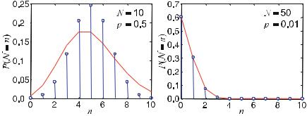
|
2 Fundamentals of X-ray Physics |
Fig. . . Comparison between binomial and Poisson distribution density functions. The binomial density function is given by the vertical lines; the Poisson density function is given by the solid line, although the Poisson process is also discrete. Left: Ten coin flipping experiments with p = . . Right: Fifty fast electrons interacting with the target medium creating an X-ray photon with a probability of p = .
p decreases, for example, let N = be the number of fast electrons and p = . be the e ciency of successful interaction in the anode material, then the binomial and Poisson model result in approximately the same distribution density function as illustrated in the right hand figure.
As shown above for the binomial density function, the probability values for the Poisson process must also in total be . With the Taylor expansion for the exponential function, it can be verified that
|
P |
|
n |
|
|
n |
n |
e− |
n |
|
e− |
n |
( |
n |
n |
|
e− |
n |
n |
|
. |
( . ) |
n = |
(N = |
) = |
n = ( |
n!) |
|
|
= |
n = |
n!) |
|
= |
e+ |
|
= |
||||||||
|
|
|
|
|
|
|
|
|
|
|
|
|
|
|
|
|
|
|||||
2.6.2 |
|
|
|
|
|
|
|
|
|
|
|
|
|
|
|
|
|
|
|
|
|
|
Statistical Properties of the X-ray Detector |
|
|
|
|
|
|
|
|
|
|
||||||||||||
Reviewing the X-ray detector types explained in |
|
Sect. . in terms of their statis- |
||||||||||||||||||||
tics, it becomes clear that the X-ray photon detections via the photoelectric e ect
can also be seen as statistically independent processes. In statistics, such detectors are called Bernoulli detectors. Let p, with p , be the probability that entering X-ray quanta ionizes a xenon atom of the detector. It has been derived in the previous section that X-ray quanta leaving the X-ray tube are Poisson-distributed. Therefore, the detection process must be modeled for a Bernoulli detector, which receives Poisson-distributed quanta.
The probability that n quanta are detected, if N quanta enter the detector, is
given by the conditional probability |
|
|
|
|
|
|
|
|
|||||||
PD n N |
- |
|
N |
|
pn |
( |
|
− |
p |
) |
N−n |
for n |
= |
, , . . . , N . |
( . ) |
n |
|||||||||||||||
( |
. |
|
|
|
|
|
for n |
N |
|
||||||
) = / |
|
|
|
|
|
|
|
|
|
|
|
|
|
|
|
|
. |
|
|
|
|
|
|
|
|
|
|
|
|
|
|
|
0 |
|
|
|
|
|
|
|
|
|
|
|
|
|
|
|
|
|
|
|
|
|
|
|
|
|
|
|
|
|
|
|
|
|
|
|
|
|
|
|
|
|
|
|
|
|
|
|
|
|
|
|
|
|
|
|
|
|
|
|
|
|
|
|
|
|
2.6 |
|
|
X-ray Photon Statistics |
|
||||||||||||||||
Since the source is modeled by the Poisson distribution, |
|
|
|
|
|
|
|
|
|
|
|
|
|
|
|
|
|
|
|
|
|
|
|
||||||||||||||||||||||||||||||||||||||||||||||||
|
|
|
|
|
|
|
|
|
|
|
|
PS (N = N) = ( |
n |
N |
|
|
|
|
n |
|
|
|
|
|
|
|
|
|
|
|
|
|
|
|
|
|
|
|
|
|
|
|
|
|
|
||||||||||||||||||||||||||
|
|
|
|
|
|
|
|
|
|
|
|
|
N)! |
|
e− |
|
|
|
|
, |
|
|
|
|
|
|
|
|
|
|
|
|
|
|
|
|
|
|
|
|
( . ) |
|
|||||||||||||||||||||||||||||
this term must be multiplied with ( . ). In this way, the probability of a Bernoulli |
|
||||||||||||||||||||||||||||||||||||||||||||||||||||||||||||||||||||||
detection of n quanta of a Poisson source can be expressed as |
|
|
|
|
|
|
|
|
|
|
|
|
|
|
|
|
|||||||||||||||||||||||||||||||||||||||||||||||||||||||
|
|
|
|
|
|
|
|
|
|
|
|
|
|
|
|
|
|
|
|
|
|
|
|
|
|
|
|
|
|
|
|
n |
|
N |
|
|
|
|
|
|
n N |
|
|
|
|
|
n |
|
|
|
|
|
|
N |
|
n |
|
|
|
|
|||||||||||
PSD |
(N = |
n |
) = |
N =n PS |
( |
N |
) |
PD |
|
|
n |
N |
) = |
N =n ( |
N)! |
|
|
|
e− |
|
|
|
|
|
n |
|
|
|
p |
|
( |
|
− |
p |
) |
|
− |
|
|
|
|
|
|||||||||||||||||||||||||||||
|
|
|
|
|
|
|
|
|
|
(N |
|
|
|
|
|
|
|
|
|
|
N |
|
|
|
|
|
|
|
|
|
|
|
|
|
|
|
|
|
|
|
|
|
|
|
|
||||||||||||||||||||||||||
|
|
|
|
|
−n |
|
|
|
n |
|
|
|
|
|
N N |
|
|
|
|
|
|
|
|
|
|
|
n |
|
|
|
|
n |
|
|
|
|
|
N−n |
|
|
|
|
|||||||||||||||||||||||||||||
|
|
|
|
e |
|
|
|
N =n ( N)! |
|
|
|
|
|
|
|
|
|
|
|
|
|
|
|
|
|
|
|
|
|
|
|
|
|
|
|
|
|
|
|
|
|
|
|
|
|
p |
|
|
|
|
p |
|
|
|
|
|
|
|
|
|
|||||||||||
|
|
|
|
|
|
|
|
|
|
|
|
|
|
|
|
|
|
|
|
|
|
|
|
n! |
|
|
|
|
|
|
|
|
|
|
|
|
|
|
|
|
|
|
|
|
|
|
|
|
|
|
|
|
|
||||||||||||||||||
|
|
|
|
|
|
|
|
|
|
|
|
|
|
|
|
|
|
|
|
|
|
|
|
|
|
|
|
|
|
|
|
|
|
|
|
|
|
|
|
|
|
|
|
|
|
|
|
|
|
|
|
|
|
|
|
|
|
|
|||||||||||||
|
|
|
= |
|
|
|
|
|
|
|
|
|
|
|
|
( − ) ( − ( − )) |
|
|
|
|
( − ) |
|
|
|
|
( . ) |
|
||||||||||||||||||||||||||||||||||||||||||||
|
|
|
e |
− |
n |
|
|
n |
|
|
n |
|
|
|
n |
|
|
N − n pn |
|
|
p N − n |
|
|
|
|
|
|
|
|
|
|
|
|
|
|||||||||||||||||||||||||||||||||||||
|
|
|
|
|
|
|
|
|
|
|
|
|
|
|
|
|
|
|
|
|
|
|
|
|
|
|
|
|
|
|
|
|
|
|
|
|
|
|
|
|
|
|
|
|
|
|
|
|
|
|
|
|
|
|
|
|
|
|
|
|
|||||||||||
|
|
|
|
|
|
|
N =n |
|
|
|
|
|
|
|
|
|
|
|
|
|
|
|
|
|
N |
|
|
|
n !n! |
|
|
|
|
|
|
|
|
|
|
|
|
|
|
|
|
|
|
|
|
|
|
||||||||||||||||||||
|
|
|
|
|
|
|
|
|
|
|
|
|
|
|
|
|
|
|
|
|
|
|
|
|
|
|
|
|
|
|
|
|
|
|
|
|
|
|
|
|
|
|
|
|
|
|
|
|
|
|
|
|
|
|
|
||||||||||||||||
|
|
|
= |
|
|
|
|
|
|
|
( ) |
|
|
|
n |
|
|
|
|
|
) |
|
|
|
|
|
|
|
|
N |
|
n |
|
|
|
|
|
|
|
|
|
|
|
|
|
|
|
|
|
|
|
|
|
|
|
|
|
|
|
|
|
|
|
||||||||
|
|
|
|
|
|
|
|
|
|
( |
|
|
|
|
|
|
|
|
|
|
|
|
|
|
|
− |
|
|
|
|
|
|
|
|
|
|
|
|
|
|
|
|
|
|
|
|
|
|
|
|
|
|
|
|
|
|
|
|
|
||||||||||||
|
|
|
|
e |
−n |
|
|
|
pn |
|
|
|
|
|
|
|
|
|
|
|
|
|
|
p n( − ) |
|
|
|
|
|
|
|
|
|
|
|
|
|
|
|
|
|
|
|
|
|
|
|
|
|
|
|||||||||||||||||||||
|
|
|
|
|
|
|
N =n ( |
|
|
|
|
|
) |
|
|
N |
|
|
|
|
n !n! |
) |
|
|
|
|
|
|
|
. |
|
|
|
|
|
|
|
|
|
|
|
|
|
|
|
|
|
|
|
|
|
|
|
|
|
|
|
||||||||||||||
|
|
|
|
|
|
|
|
|
|
|
|
|
|
|
|
|
|
|
|
|
|
|
|
|
|
|
|
|
|
|
|
|
|
|
|
|
|
|
|
|
|
|
|
|
|
|
|
|
|
|
|
|
|
|
|||||||||||||||||
|
|
|
= |
|
|
|
|
|
|
|
|
|
|
|
|
|
|
|
|
|
|
|
|
|
|
|
|
|
|
|
|
|
|
|
|
|
|
|
|
|
|
|
|
|
|
|
|
|
|
|
|
|
|
|
|
|
|
|
|
|
|
|
|
|
|
|
|
|
|
||
In the last part of ( . ), terms that do not include the number of entering pho- |
|
||||||||||||||||||||||||||||||||||||||||||||||||||||||||||||||||||||||
|
|
|
|
|
|
|
|
|
|
|
|
|
|
|
|
|
|
|
( |
|
|
|
|
|
− |
|
) |
|
|
|
|
|
|
|
|
|
|
|
|
|
|
|
|
|
|
|
|
|
|
|
|
|
|
|
|
|
|
|
|
|
|
|
|
|
|
|
|||||
tons, N, are factored out of the sum. Thus, one obtains |
|
|
|
|
|
|
|
|
|
|
|
|
|
|
|
|
|
|
|
|
|
|
|
|
|||||||||||||||||||||||||||||||||||||||||||||||
|
|
|
PSD |
|
|
|
|
|
n |
|
|
|
|
e− |
n |
|
( |
pn |
|
n |
|
|
|
|
(( |
|
|
|
|
|
p n |
|
N −n |
. |
|
|
|
|
|
|
( . ) |
|
|||||||||||||||||||||||||||||
|
|
|
(N = |
|
) = |
|
|
|
|
|
|
|
n! ) |
|
|
N =n |
|
|
−N ) |
|
n)! |
|
|
|
|
|
|
|
|
|
|
|
|||||||||||||||||||||||||||||||||||||||
|
|
|
|
|
|
|
|
|
|
|
|
|
|
|
|
|
|
|
|
|
|
|
|
|
|
|
|
|
|
|
|
|
|
( |
|
|
|
− |
|
) |
|
|
|
|
|
|
|
|
|
|
|
|
|
|
|
|
|
||||||||||||||
Shifting the sum index gives |
|
|
|
|
|
|
|
|
|
|
|
|
|
|
( |
|
|
|
|
|
n |
|
|
|
|
(( |
|
|
|
|
|
) |
N |
|
|
|
|
|
|
|
|
|
|
|
|
|
|||||||||||||||||||||||||
|
|
|
|
|
|
|
|
|
|
|
|
|
|
|
|
|
|
|
|
|
|
|
n |
pn |
|
|
|
|
|
|
|
p n |
|
|
|
|
|
|
|
|
|
|
|
|
|
||||||||||||||||||||||||||
|
|
|
|
PSD |
(N = |
n |
) = |
|
e− |
|
|
|
|
|
n! ) |
|
N = |
|
|
|
−N)! |
|
|
|
|
. |
|
|
|
|
|
|
|
( . ) |
|
||||||||||||||||||||||||||||||||||||
|
|
|
|
|
|
|
|
|
|
|
|
|
|
|
|
|
|
|
|
|
|
|
|
|
|
|
|
|
|
|
|
|
|
|
|
|
|
|
|
|
|
|
|
|
|
|
|
|
|
|
|
|
|
|
|
|
− |
p |
n |
|
|||||||||||
The sum in ( . ) is the Taylor expansion of the exponential function e( |
) |
. |
|
||||||||||||||||||||||||||||||||||||||||||||||||||||||||||||||||||||
Ultimately, one obtains |
|
|
|
|
|
|
|
|
|
|
|
|
|
|
|
|
|
|
|
|
|
|
|
|
|
|
|
|
|
|
|
|
|
|
|
|
|
|
|
|
|
|
|
|
|
|
|
|
|
|
|
|
|
|
|
|
|
|
|
|
|
|
|
||||||||
|
|
|
|
|
|
|
|
|
|
|
|
|
|
|
|
|
|
|
|
|
|
|
|
|
|
|
|
|
|
n |
|
pn |
|
n |
|
|
|
|
|
|
|
p |
n |
|
|
|
|
|
|
|
|
|
|
|
|
|
|
|
|
|
|
|
|||||||||
|
|
|
|
|
|
|
|
PSD |
(N = |
|
n |
) = |
e− |
|
|
( nn! ) |
|
e( |
|
|
− |
|
) |
|
|
pn |
|
|
|
|
|
|
|
|
|
|
|
|
|
|
|
|
|
||||||||||||||||||||||||||||
|
|
|
|
|
|
|
|
|
|
|
|
|
|
( |
pn |
|
|
|
|
n |
|
|
|
|
|
n |
|
|
|
|
|
|
|
|
|
|
|
|
|
|
|
|
|
|
|
|
|||||||||||||||||||||||||
|
|
|
|
|
|
|
|
|
|
|
|
|
|
|
|
|
|
|
|
|
|
|
|
= |
|
n! )n e− |
|
|
e+ |
|
|
|
|
e− |
|
|
|
|
|
|
|
|
|
|
|
|
|
|
|
|
|
( . ) |
|
||||||||||||||||||
|
|
|
|
|
|
|
|
|
|
|
|
|
|
|
|
|
|
|
|
|
|
|
|
( |
pn |
|
|
|
|
pn |
|
|
|
|
|
|
|
|
|
|
|
|
|
|
|
|
|
|
|
|
|
|
|
|
|
|
|
|
|
|
|
|
|||||||||
|
|
|
|
|
|
|
|
|
|
|
|
|
|
|
|
|
|
|
|
|
|
|
|
|
|
|
|
n! ) |
e− |
|
. |
|
|
|
|
|
|
|
|
|
|
|
|
|
|
|
|
|
|
|
|
|
|
|
|
|
|
|
|
|
|||||||||||
=
Equation ( . ) reveals that the number of Bernoulli-detected X-ray quanta of a Poisson source is again a Poisson-distributed random variable. The final result is merely scaled by the detection probability, p, i.e., the e ciency of the detector.
Equation ( . ) is exceedingly important because it explains why X-ray quanta show Poisson statistics after traveling through an absorbing object. Obviously, the attenuation processes inside the object are guided by binomial statistics, since the mechanisms for absorption are the same as those inside the detector. The statistical chain from generation of the quanta inside the X-ray tube, via the attenuation inside the object of interest, to the measurement by the X-ray detector, is called a cascaded Poisson process.

2 Fundamentals of X-ray Physics
2.6.3
Statistical Law of Attenuation
Similar to the situation in Sect. . , the traveling length, s, of X-ray quanta through an object of interest is subdivided into m slices. In Fig. . , the geometric situation for a statistical model of the attenuation process is given. The subdivisions are non-overlapping, and the attenuation processes are assumed to be statistically independent.
An X-ray quantum arriving at position η has the probability
|
pt |
|
μ η η , |
( . ) |
|||||
|
|
|
|
turn, the probability |
|
||||
of passing the object interval and,=in − |
( ) |
|
|
|
|||||
|
|
pa |
μ η η , |
( . ) |
|||||
of being absorbed in that interval. |
Generally, the transmission probability of the |
||||||||
|
= |
( ) |
|
|
|
|
|||
X-ray quantum running through interval i is given by |
|
||||||||
with |
pt,i − μ(i |
η) η , |
( . ) |
||||||
|
η = |
s |
|
|
|
η = i |
s |
|
|
|
|
and |
|
. |
( . ) |
||||
|
m |
m |
|||||||
In the limit m , ( . ) becomes exact. Since the intervals are disjoint and the attenuation processes are assumed to be statistically independent, the transmission probability for the entire traveling length, s, is given by
|
|
|
|
|
m |
|
|
|
|
|
|
|
|
|
pt,s |
1 |
pt,i . |
|
|
|
|
|
( . ) |
||
|
|
|
|
|
i = |
|
|
|
|
|
|
|
The logarithm of ( . ) gives |
|
|
|
|
|
|
|
|
|
|
|
|
ln |
pt,s |
lim |
|
m |
ln μ |
i |
s |
|
s |
. |
( . ) |
|
|
|
|
||||||||||
|
|
m |
|
m |
||||||||
( |
) = |
m i = |
− |
|
|
|
|
|||||
|
|
|
|
|
||||||||
Fig. . . Subdivision of the X-ray quanta traveling length into the m disjoint, statistically independent intervals of thickness η
2.6 X-ray Photon Statistics |
|
Due to the limit in ( . ), the Taylor expansion for the logarithm in ( . ) can be truncated after the linear term, such that
( |
|
) = − |
|
m |
|
|
|
|
|
|
|
|
|
|
|
|
|
|
|
|
|||||
pt,s |
lim |
μ |
i |
s |
s |
( . ) |
||||||
ln |
|
|
|
|
||||||||
|
|
|
m i = |
|
|
|
m |
|
m |
|
||
is obtained. However, due to the limit, the right-hand side of ( . ) is essentially the integral
ln(pt,s) = − |
s |
|
∫ μ (η) dη . |
( . ) |
This means, the probabilities of X-ray quantum transmission and absorption during traveling through the entire object are given by
|
|
|
|
|
|
|
s |
|
|
|
|
|
|
|
|
|
|
|
|
|
|
|
|
|
|
|
|
s |
|
|
|
|
|
pt,s |
|
− ∫ μ(η)dη |
and |
pa,s |
|
|
|
|
|
− ∫ μ(η)dη |
( . ) |
||||||||||||||||||
|
|
|
e |
|
|
|
|
|
|
|
|
|
|
e |
|
|
|
|
|||||||||||||
respectively. The |
probability that n N quanta are transmitted, if N quanta are |
||||||||||||||||||||||||||||||
|
= |
|
|
|
|
|
|
|
|
|
|
|
|
|
|
|
|
|
= − |
|
|
|
|
|
|
|
|||||
leaving the X-ray source, is again |
given by the Bernoulli distribution function, |
||||||||||||||||||||||||||||||
|
|
< |
|
|
|
pn |
( − p)N−n , |
|
|
|
|||||||||||||||||||||
|
|
|
|
P (N = n) = n |
|
|
( . ) |
||||||||||||||||||||||||
|
|
|
|
|
|
|
|
|
|
|
|
|
|
|
|
N |
|
|
|
|
|
|
|
|
|
|
|
|
|
||
with an expectation value, |
|
|
|
|
|
|
|
|
|
|
|
|
|
|
|
|
|
|
|
|
|
|
|
|
|
|
|||||
|
|
|
|
|
|
|
= |
|
[N] = |
|
N |
N |
|
(N = |
|
|
) |
|
|
|
|
||||||||||
|
|
|
|
n |
E |
|
P |
n |
, |
|
|
( . ) |
|||||||||||||||||||
|
|
|
|
|
|
|
|
|
|
|
|
|
|
|
|
n = |
|
|
|
|
|
|
|
|
|
|
|
|
|
||
that can be calculated via the definition of the binomial series, i.e., |
|
||||||||||||||||||||||||||||||
|
|
|
N |
|
( |
|
|
) = |
|
N |
|
|
N |
|
|
|
|
|
= ( |
|
|
+ |
|
) |
|
|
|||||
|
|
|
P |
n |
|
pn qN−n |
p |
q |
N , |
( . ) |
|||||||||||||||||||||
|
|
n = |
|
|
|
|
|
|
n = |
|
|
n |
|
|
|
|
|
|
|
|
|
|
|
|
|
|
|
|
|||
|
Applying the operator p |
|
∂ |
∂p to both sides of ( . ) yields |
|
||||||||||||||||||||||||||
with p + q = . |
|
p |
∂ |
|
|
|
N |
P |
|
n |
|
|
|
|
ċ |
|
N |
|
N |
|
pnpn − qN − n |
|
|||||||||
|
|
|
( |
|
|
|
|
|
|
|
|
|
|||||||||||||||||||
|
|
|
∂p |
|
|
) = |
|
n |
|
|
|
|
|
|
|
|
|
|
|||||||||||||
|
|
|
|
n = |
|
|
|
|
|
|
|
n = |
|
|
|
|
|
|
|
|
|
|
|
||||||||
|
|
|
|
|
|
|
|
|
|
|
|
|
|
|
|
|
|
N |
|
N |
|
|
− |
|
|
|
|
|
( . ) |
||
|
|
|
|
|
|
|
|
|
|
|
|
|
|
|
|
|
|
|
n |
N −n |
|
||||||||||
|
|
|
|
|
|
|
|
|
|
|
|
|
|
|
|
|
|
|
|
|
|
|
|
||||||||
|
|
|
|
|
|
|
|
|
|
|
|
|
|
= n = n n pN q |
. |
|
|
|
|
||||||||||||
|
|
|
|
|
|
|
|
|
|
|
|
|
|
= pN(p + q) |
|
|
|
|
|
|
|
|
|||||||||
Since the middle row of ( . ) is the explicit calculation of the expectation value in ( . ) and p + q = , it has been shown that
|
[N] = |
|
N |
N |
|
|
(N = |
|
) |
|
|
|
|
||||
E |
n |
= |
P |
n |
|
|
|
|
|||||||||
|
|
|
n = |
|
|
|
|
|
|
|
|
|
|
|
|
|
( . ) |
|
|
|
N |
|
|
N |
|
|
( |
|
− |
) |
|
= |
|
||
|
|
|
= |
n |
pn |
|
N − n |
Np . |
|||||||||
|
|
|
|
|
|
|
|
|
p |
|
|||||||
n = |
n |
|

|
2 |
Fundamentals of X-ray Physics |
|
|
|
|
|
|
|
|
|
|
|
|
This means that one has an ideal detector if p |
|
, and the detector is switched o |
||||||||||
|
if p |
|
(Epstein ). For the expectation |
value of the X-ray quanta number, one |
|||||||||
|
|
|
= |
|
|
|
|
|
|
||||
|
obtains |
|
|
|
|
|
|
|
|
|
|
||
|
|
= |
|
|
|
|
s |
|
|
|
|
|
|
|
|
|
n |
Npt,s |
|
− ∫ μ(η)dη |
|
|
( . ) |
||||
|
|
|
N e |
|
|
|
|
||||||
|
when ( . ) is substituted into (=. ). It |
=has already been mentioned that the num- |
|||||||||||
|
ber of X-ray quanta is proportional to the radiation intensity. With n |
I |
( |
s |
) |
and |
|||||||
|
N |
|
I( ), ( . ) finally reads |
|
|
s |
|
|
|
|
|
|
|
|
|
|
|
|
− ∫ μ(η)dη |
|
|
( . ) |
|||||
|
|
|
I(s) = I( )e |
|
|
. |
|
|
|||||
The statistical discussion of the attenuation process also leads us to Lambert–Beer’s law. It should be noted that the same result is obtained if the Poisson distribution function ( . ) is used instead of the binomial distribution function in ( . ).
2.6.4
Moments of the Poisson Distribution
To evaluate the image quality of the CT imaging process quantitatively, one has to discuss the moments of the Poisson distribution function. The first moment of the Poisson distribution is given by
μ |
= |
E |
[N] = N |
P |
(N = |
n |
) |
, |
( . ) |
|
|
|
n |
|
|
|
|
|
|
i.e., the expectation value, μ, of the number of X-ray quanta assigned with the random variable N. Further, the second central moment is given by
σ |
= |
|
2(N − |
|
) |
3 = (N − |
|
) |
P |
(N = |
|
) |
|
|
|
E |
|
μ |
|
n |
μ |
|
|
n |
|
, |
( . ) |
||
|
|
|
|
|
|
|
|
|
|
|
|
|
|
i.e., the variance, σ , of the distribution. The square root of the variance is the standard deviation, σ.
An important value for quantitative signal or image quality evaluation is the
signal-to-noise ratio, defined as the ratio, |
|
|
||
|
SNR(N) = σ |
, |
( . ) |
|
|
|
μ |
|
|
between signal mean |
and standard deviation. |
|
|
|
The expectation value of a binomially distributed random variable has already been used in the previous section. The result of ( . ) was E[N] = Np. To calculate
The mean is an estimate of the expectation value only. However, in this book the symbol is the same.
2.6 X-ray Photon Statistics |
|
the expectation value of a Poisson-distributed random variable, it is started with the same term,
|
|
N |
|
(N = |
|
) |
|
|
E |
[N] = |
P |
n |
, |
( . ) |
|||
|
n = |
|
|
|
|
|
|
|
and utilized the definition of the Poisson distribution function ( . ) such that
|
[N] = |
|
n n |
|
n |
|
= |
|
|
|
n n |
|
n |
n − |
|
|||||
E |
|
|
|
e− |
|
n |
|
|
( n!) |
e− |
|
|
|
|||||||
|
n = n ( n!) |
|
|
|
|
n = n |
|
|
|
|
||||||||||
|
= |
|
n |
|
|
n |
|
|
n= |
|
|
n |
|
|
n |
|
|
|
||
|
e− |
|
|
n ( |
n!) |
|
e− |
|
|
n |
( n ) |
! |
( . ) |
|||||||
|
|
|
n = |
|
|
|
|
n = |
||||||||||||
|
= |
|
|
n |
|
n |
|
|
= |
|
|
n |
n ( − ) |
|
||||||
|
n e− |
|
( ) |
|
n e− e+ |
= |
n . |
|
||||||||||||
|
|
n = |
( n )! |
|
|
|
|
|
||||||||||||
Obviously, the parameter
E [N] = n
is the expectation value. This is consistent with the result of ( . ), because n = Np and, within the limits N and p , the Bernoulli distribution transforms to the Poisson distribution function.
The variance of a Poisson-distributed random variable can also be calculated explicitly. Starting again with
|
2(N − |
|
) |
|
(N − |
|
) |
|
(N = |
|
) |
|
|
|
3 = |
|
P |
|
|
||||||
E |
|
μ |
|
n = |
|
μ |
|
|
n |
|
( . ) |
|
|
|
|
|
|
|
|
|
|
|
|
|
and substituting the definition of the Poisson distribution function and the result
of ( . ), one derives
E 2(N − μ) 3
= |
|
( |
n |
− |
n |
) |
|
( |
n n |
e− |
n |
|
|
|
|
|
|
|
|
|
|
|
|
n |
|
|
|
|
|
|
|
|
|
|
|
|
|
|
|
|
|
|
|
|
|
n |
|
|
|
|
||||||||
n = |
|
|
|
|
n |
|
|
|
|
|
|
|
|
|
|
|
|
|
|
|
|
|
|
|
|
|
|
|
|
|
|
|
|
|
|
|
|
|
|
|
|
|
|
|
||||||||||||||
|
|
|
|
|
|
|
n!) |
|
|
|
|
|
|
|
|
|
|
|
|
|
|
|
|
|
|
|
|
|
|
|
|
|
|
|
|
|
|
|
|
|
|
|
|
|
|
|
||||||||||||
= |
|
|
& |
|
|
|
( |
n |
|
|
|
−− |
|
|
|
|
|
|
|
n |
|
|
|
+ ( ) |
|
|
|
|
|
|
|
( |
n |
|
|
' |
|
|
||||||||||||||||||||
|
n |
|
|
|
|
|
|
|
|
|
|
|
|
|
|
|
|
|
|
|
|
|
|
|
|
|
|
|
|
|||||||||||||||||||||||||||||
|
e− |
|
|
|
|
n = n |
|
n!) |
|
|
n n = n ( |
|
|
n!) |
|
|
|
|
n |
|
|
|
n = |
n!) |
|
|
|
|
|
|||||||||||||||||||||||||||||
= |
|
n |
& |
|
|
|
|
|
|
n |
n |
|
|
−n |
( ) |
|
|
|
|
|
n |
+ ( ) |
|
|
|
|
n |
' |
|
|
|
|
|
|
|
|||||||||||||||||||||||
|
|
|
|
|
|
|
|
|
|
|
|
|
|
|
|
|
|
|
|
|
|
|
|
|
|
|
|
|
|
|
|
|
|
|
|
|
|
|
|
|
|
|
|
|||||||||||||||
|
e− |
|
|
|
|
n n = n |
( n ) |
! |
|
n |
|
|
|
|
|
e+ |
|
|
|
|
|
n |
|
|
|
|
e+ |
|
|
|
|
|
|
|
|
|
|
|
|
|
||||||||||||||||||
= |
|
n |
& |
|
|
|
( |
( − )n |
|
− |
|
( |
|
|
|
|
|
|
|
|
|
n |
|
+ ( |
|
|
|
|
) |
|
|
|
|
n |
' |
|
|
|
|
|||||||||||||||||||
e− |
|
|
|
|
|
n |
|
+ )n |
( |
n )! |
|
|
n |
)n |
e+ |
|
|
|
n |
|
|
|
e+ |
|
|
|
|
|
( . ) |
|||||||||||||||||||||||||||||
|
|
|
|
|
n n = |
|
|
|
|
|
|
|
|
|
|
|
|
|
|
|
|
|
|
|
|
|
|
|
|
|
|
|
|
|||||||||||||||||||||||||
= |
|
n |
& |
|
|
|
|
|
|
n |
|
( |
|
) |
|
|
|
|
|
n |
|
|
|
− |
|
( |
|
) |
|
|
|
|
|
n |
+ ( |
|
|
) |
n |
' |
||||||||||||||||||
e− |
|
|
|
|
|
|
|
( |
|
) |
|
+ |
|
|
|
|
( |
|
|
) |
|
|
|
n |
|
e+ |
|
|
|
n |
e+ |
|||||||||||||||||||||||||||
|
|
|
|
|
n n = n ( |
|
n )! |
|
|
n n = |
( |
|
|
n )! |
|
|
|
|
|
|
|
|
|
|
|
|
|
|
|
|
|
|
||||||||||||||||||||||||||
=e−n 4(n ) e+n + n e+n − (n ) e+n + (n ) e+n 5
=e−n e+n 4(n ) + n − (n ) + (n ) 5 = n .
|
2 Fundamentals of X-ray Physics |
|
|
|
|
|
|
|
|
|
|
|
|
|
|
|
|
|
|
|
|
|
|
|
|
|
|
|
|
|
|
|
|
|
|
|
|
|
|
|
|
|
|
|
|
|
|
|
|
|||||||||||||
|
The results of ( . ) and ( . ) characterize the Poisson distribution. Obviously, it |
|||||||||||||||||||||||||||||||||||||||||||||||||||||||||||||
|
holds that |
|
|
|
|
|
|
|
|
|
|
|
|
|
|
|
|
|
|
|
|
|
|
|
|
|
|
|
|
|
|
|
|
|
|
|
|
|
|
|
|
|
|
|
|
|
|
|
|
|
|
|
|
|
|
|
|
|
|
|
|
|
|
|
|
|
|
|
|
|
|
|
|
|
|
|
|
|
|
|
|
|
μ |
|
|
|
|
σ , |
|
|
|
|
|
|
|
|
|
|
|
|
|
|
|
|
|
|
|
|
|
|
|
|
|
|
|
( . ) |
|||||||||
|
which means that the expectation value=equals the variance of the random variable |
|||||||||||||||||||||||||||||||||||||||||||||||||||||||||||||
|
|
|
|
|
|
|
|
|
E |
|
|
|
|
|
|
|
|
|
E |
|
|
|
|
|
|
|
|
|
|
|
|
μ . |
|
|
|
|
|
|
|
|
|
|
|
|
|
( . ) |
||||||||||||||||
|
For the signal-to-noise ratio of |
Poisson-distributed signals, like X-ray radiation, one |
||||||||||||||||||||||||||||||||||||||||||||||||||||||||||||
|
|
[N] = |
|
|
|
|
2(N − ) |
|
|
3 |
|
|
|
|
|
|
|
|
|
|
|
|
|
|
|
|
|
|
||||||||||||||||||||||||||||||||||
|
obtains |
|
|
|
|
|
|
|
|
|
|
|
|
|
|
|
|
|
|
|
|
|
|
|
|
|
|
|
|
|
|
|
|
|
|
6 |
|
|
|
|
|
|
|
|
|
|
|
|
|
|
|
|
|
|
|
|
||||||
|
|
|
|
|
|
|
|
|
|
|
|
|
|
|
|
|
|
|
|
|
|
|
|
|
|
|
|
|
|
|
|
|
|
|
|
|
|
|
|
|
|
|
|
|
|
|
|
|
|
|
|
|
|
|
||||||||
|
|
|
|
|
|
|
|
SNR |
|
|
|
|
|
|
|
|
|
|
|
n |
|
|
|
|
|
|
|
|
. |
|
|
|
|
|
|
|
|
|
|
|
|
( . ) |
||||||||||||||||||||
|
|
|
|
|
|
|
|
|
|
|
|
|
|
|
|
|
|
|
|
|
|
|
|
n |
|
|
|
|
|
|
|
|
|
|
|
|
||||||||||||||||||||||||||
|
|
|
|
|
|
|
|
|
|
|
|
|
|
|
|
|
|
|
|
|
|
|
|
|
|
|
|
|
|
|
|
|
|
|
|
|
||||||||||||||||||||||||||
|
|
|
|
|
|
|
|
|
|
|
|
|
|
|
|
|
|
|
|
n |
|
|
|
|
|
|
|
|
|
|
|
|
|
|
|
|
|
|||||||||||||||||||||||||
|
The signal-to-noise ratio increases(Nwith) = 6the square= |
root of the number of quanta. |
||||||||||||||||||||||||||||||||||||||||||||||||||||||||||||
|
Considering ( . ) and ( . ), the signal-to-noise ratio is proportional to the square |
|||||||||||||||||||||||||||||||||||||||||||||||||||||||||||||
|
root of the X-ray tube current. |
|
|
|
|
|
|
|
|
|
|
|
|
|
|
|
|
|
|
|
|
|
|
|
|
|
|
|
|
|
|
|
|
|
|
|
|
|
|
|
|
|
|
|
|
|
|
|
|
|
|
|
|
|
||||||||
|
2.6.5 |
|
|
|
|
|
|
|
|
|
|
|
|
|
|
|
|
|
|
|
|
|
|
|
|
|
|
|
|
|
|
|
|
|
|
|
|
|
|
|
|
|
|
|
|
|
|
|
|
|
|
|
|
|
|
|
|
|
|
|
|
|
|
Distribution for a High Number of X-ray Quanta |
|
|
|
|
|
|
|
|
|
|
|
|
|
|
|
|
|
|
|||||||||||||||||||||||||||||||||||||||||||
|
For a high number of quanta, the factorial in ( . ) can be approximated by the |
|||||||||||||||||||||||||||||||||||||||||||||||||||||||||||||
|
Stirling equation, |
|
|
|
|
|
|
|
|
|
|
|
n! nn e−n 6 |
|
|
|
|
|
|
|
|
|
|
|
|
|
|
|
|
|
|
|
|
|
|
|
|
|
|
|
|
|
||||||||||||||||||||
|
|
|
|
|
|
|
|
|
|
|
|
|
. |
|
|
|
|
|
|
|
|
|
|
|
|
|
|
|
|
|
|
|
( . ) |
|||||||||||||||||||||||||||||
|
In this case one obtains |
|
|
|
|
|
|
|
πn |
|
|
|
|
|
|
|
|
|
|
|
|
|
|
|
|
|
|
|
||||||||||||||||||||||||||||||||||
|
|
|
|
|
|
|
|
|
|
|
|
|
|
|
n |
n |
|
|
|
|
n |
|
|
|
|
|
|
|
|
|
|
|
|
|
|
|
n |
|
|
n |
|
|
|
|
|
|
n |
|
|
|||||||||||||
|
P |
(N = |
n |
) = |
( |
n!) |
|
|
e− |
|
|
|
|
|
|
|
nn e(−n |
|
|
) |
|
|
|
e− |
|
|
|
|
||||||||||||||||||||||||||||||||||
|
|
|
|
|
|
|
|
|
|
|
πn |
|
|
|
|
|||||||||||||||||||||||||||||||||||||||||||||||
|
|
|
|
|
|
|
|
|
|
|
|
|
|
|
|
|
|
|
|
|
|
|
|
|
|
|
|
|
|
|
|
|
|
|
|
n |
|
|
|
|
|
|
|
|
|
|
|
|||||||||||||||
|
|
|
|
|
|
|
|
|
|
|
|
|
|
|
|
|
|
|
|
|
|
|
|
|
|
n |
|
6 |
|
|
|
|
|
|
|
|
|
|
|
|||||||||||||||||||||||
|
|
|
|
|
|
|
|
|
|
|
|
|
|
|
|
|
|
|
|
e |
−(n −n) |
|
|
|
|
|
|
|
|
|
|
|
|
|
|
|
|
|
|
|
( . ) |
|||||||||||||||||||||
|
|
|
|
|
|
|
|
|
= 6 |
|
|
|
|
|
|
|
|
|
|
|
|
|
|
|
|
|
|
|
|
|
|
n |
|
|
|
|
|
|
|
|
|
|
|
|
|
|
||||||||||||||||
|
|
|
|
|
|
|
|
|
πn |
|
|
|
|
|
|
|
|
|
|
|
|
|
|
|
|
|
|
|
|
|
|
|
|
|
|
|
|
|
||||||||||||||||||||||||
|
|
|
|
|
|
|
|
|
|
|
|
|
|
|
|
|
|
|
|
|
|
|
|
|
|
|
|
|
|
|
|
|
|
|
|
|
|
|
|
|
|
|||||||||||||||||||||
|
|
|
|
|
|
|
|
|
|
|
|
|
|
|
|
|
|
|
|
|
|
|
|
|
|
|
|
|
|
|
|
|
|
|
|
|
|
n |
+ |
|
|
|
|
|
|
|
|
|||||||||||||||
|
|
|
|
|
|
|
|
|
|
|
|
|
|
|
|
|
|
|
|
|
|
|
e |
−(n −n) |
|
|
|
|
n |
|
|
|
|
|
|
|
|
|
|
|
|
|
||||||||||||||||||||
|
|
|
|
|
|
|
|
|
|
|
|
|
|
|
|
|
|
|
|
|
|
|
|
|
|
|
|
|
|
|
|
|
|
|
|
|
|
|
|
|
|
|
n |
|
|
|
|
|
|
|
|
|
|
|
|
|
|
|
||||
|
|
|
|
|
|
|
|
|
|
|
|
|
|
|
|
πn |
|
|
|
|
|
|
|
|
|
|
|
|
|
|
|
|
|
|
|
|
|
|
|
|
|
|
|
|
|
|
|
|
|
|
|
|||||||||||
|
as an approximation of the Poisson= 6 distribution density function. Analogous to the |
|||||||||||||||||||||||||||||||||||||||||||||||||||||||||||||
|
derivative of ( . ), exp |
|
ln |
(ċ)) |
is applied onto the bracketed term in the last row of |
|||||||||||||||||||||||||||||||||||||||||||||||||||||||||
|
|
|
|
that |
|
|
|
|
|
|
|
|
|
|
|
|
|
|
|
|
|
|
|
|
|
|
|
|
|
|
|
|
|
|
|
|
|
|
|
|
|
|
|
|
|
|
|
|
|
|
|
|
|
|
|
|
||||||
|
equation ( . ), such |
|
( |
|
|
|
|
|
|
|
|
|
|
|
|
|
|
|
|
|
|
|
|
|
|
|
|
|
|
|
|
|
|
|
|
|
|
|
|
|
|
|
|
|
|
|
|
|
|
|
|
|
|
|
|
|
||||||
|
P |
|
|
|
|
n |
|
|
|
|
|
|
|
|
|
|
|
|
|
|
|
|
−(n |
−n) |
|
|
|
ln |
n |
n+ |
|
|
|
|
|
|
|
|||||||||||||||||||||||||
|
|
|
|
|
|
|
|
|
|
|
|
|
|
|
|
|
|
|
|
|
|
|
n |
|
|
|
|
|
|
|
||||||||||||||||||||||||||||||||
|
|
|
|
|
|
|
|
|
|
|
|
|
|
|
|
|
|
|
|
|
e |
|
|
|
|
|
|
|
|
|
|
|
|
|
e |
|
|
|
|
|
|
|
|
|
|
|
|
|
|
|
|
|
|
|
|
|||||||
|
|
|
(N = ) = |
|
|
|
|
πn |
|
|
|
|
|
|
|
|
|
|
|
|
|
|
|
|
|
|
|
|
|
|
|
|
|
|
|
|
|
|
|
|
|
|
|
|
|
|
|
|
|
|||||||||||||
|
|
|
6 |
|
|
|
|
|
−(n |
−n) |
|
|
|
n+ ln |
n |
|
|
|
( . ) |
|||||||||||||||||||||||||||||||||||||||||||
|
|
|
|
|
|
|
|
|
|
|
|
|
n |
|
|
|
||||||||||||||||||||||||||||||||||||||||||||||
|
|
|
|
|
|
|
|
|
|
|
|
|
|
|
|
|
|
|
|
|
|
|
|
|
e |
|
|
|
|
|
|
|
|
|
|
|
|
|
e |
|
|
|
|
|
|
|
|
|
|
|
|
|
|
|
|
|
. |
|
|
|||
|
|
|
|
|
|
|
|
|
|
|
|
|
|
|
|
|
πn |
|
|
|
|
|
|
|
|
|
|
|
|
|
|
|
|
|
|
|
|
|
|
|
|
|
|
|
|
|
|
|
|
|
|
|
|
|
|
|||||||
|
With the Taylor expansion of the= 6logarithm ( . ), one obtains |
|
|
|||||||||||||||||||||||||||||||||||||||||||||||||||||||||||
|
P (N = n) = |
6 |
|
|
|
|
|
|
e−( |
n |
− |
|
n |
) e |
n |
+ |
|
|
|
ln |
+ |
n −n |
|
|
|
|
|
|||||||||||||||||||||||||||||||||||
|
|
|
|
|
|
|
|
|
|
|
|
|
|
|
|
|
|
|
n |
|
|
|
|
|
||||||||||||||||||||||||||||||||||||||
|
πn |
|
|
|
|
|
|
|
|
|
|
|
|
|
|
|
|
|
|
|
|
−n |
|
( . ) |
||||||||||||||||||||||||||||||||||||||
|
|
|
|
|
|
|
6 |
|
|
|
|
|
|
|
|
|
|
|
|
|
|
|
|
|
|
|
|
|
|
|
|
n |
|
|
|
|
|
|
|
n −n |
|
|
|
n |
|
|
||||||||||||||||
|
|
|
|
|
|
|
|
|
|
|
e−( |
n |
− |
n |
) e + |
|
|
|
|
|
n |
|
− |
|
|
|
n |
|
, |
|
||||||||||||||||||||||||||||||||
|
|
|
|
|
|
|
|
|
|
|
|
|
|
|
|
|
|
|
|
|
|
|
|
|
|
|
|
|
||||||||||||||||||||||||||||||||||
|
|
|
|
|
|
πn |
|
|
|
|
|
|
|
|
|
|
|
|
|
|
|
|
|
|
|
|
|
|
|
|
|
|
|
|
||||||||||||||||||||||||||||

2.6 X-ray Photon Statistics |
|
which can be truncated after the quadratic term. As one is interested in very large numbers of X-ray quanta, n, the term (n + ) can be substituted with n, such that
P (N = n) |
6 |
|
|
n |
|
|
n |
|
|
|
n n n−n − |
n n−n |
|
|||||||||||
|
|
e−( |
|
− |
|
) e |
|
|
|
|
|
|
|
|
|
|
|
|
||||||
πn |
|
|
|
|
|
|
|
|
|
|
|
|
|
|
||||||||||
|
|
|
−( |
n |
− |
n |
) |
|
n |
− |
n |
− |
n |
|
n −n |
|
|
( . ) |
||||||
|
|
|
|
|
|
|
|
|
|
|
|
|
|
n |
|
|||||||||
= 6 |
|
|
|
|
|
|
|
|
|
|
|
|
||||||||||||
πn |
e |
|
(n −n) |
|
|
e |
|
|
|
|
e |
|
|
|
|
|
|
|
||||||
= |
6 |
|
|
|
|
|
|
|
|
|
|
|
|
|
|
|
|
|
||||||
|
|
e− |
n |
. |
|
|
|
|
|
|
|
|
|
|
|
|||||||||
πn |
|
|
|
|
|
|
|
|
|
|
|
|||||||||||||
For highly probable numbers of events, i.e., n |
|
|
n |
,norn(n |
−n |
|
) n ll , ( . ) finally |
|||||||||||||||||
transforms into |
|
|
|
|
|
|
|
|
||||||||||||||||
P (N = n) 6 πn e− |
|
n |
, |
|
|
|
|
|
( . ) |
|||||||||||||||
|
|
|
|
|
|
|
|
|
|
|
|
|
|
( |
− ) |
|
|
|
|
|
|
|
||
which is the probability density function of Gaussian distributed random variables. ( . ) is a consequence of what is called the Central Limit Theorem. T he Central Limit Theorem ensures that, regardless of the underlying distribution of mutu-
P(N = n)
0 |
.1 |
8 |
|
|
N = |
0 |
.1 |
6 |
|
|
|
0 |
.1 |
4 |
|
|
p = |
0 |
.1 |
2 |
|
|
n*= |
0 |
.1 |
0 |
|
|
|
0 |
.0 |
8 |
|
|
|
0 |
.0 |
6 |
|
|
|
0 |
.0 |
4 |
|
|
|
0 |
.0 |
2 |
|
|
|
0 |
.0 |
00 |
2 |
4 n 6 |
8 |
10 |
|
0.5 |
2 |
5 |
10- |
|
P(N = n) / |
1 0
4 .0 |
|
|
N = 10000 |
||
3 .5 |
|
|
|||
|
|
p = 0.01 |
|
||
3 .0 |
|
|
|
||
|
|
n*= 100 |
|
||
2 .5 |
|
|
|
||
|
|
|
|
||
2 .0 |
|
|
|
|
|
1 .5 |
|
|
|
|
|
1 .0 |
|
|
|
|
|
0 .5 |
|
|
|
|
|
0 |
6 0 |
8 0 |
1 0 0 |
1 2 0 |
1 4 0 |
|
|
|
n |
|
|
P(N = n) / 10-2
3 |
.0 |
|
|
|
|
|
≈ |
|
|
p = 0.01 |
|
|
N = 20000; n* = 200 |
|
|
||||||||
2 |
.5 |
|
|
|
|||||||
|
|
|
|
|
|
|
|
|
|||
2 |
.0 |
|
|
|
N = 60000; n* = 600 |
|
|
||||
1 |
.5 |
|
|
|
|
|
|||||
|
|
|
|
|
N = 100000; n* = 1000 |
|
|||||
1 |
.0 |
|
|
|
|
|
|
||||
|
|
|
|
|
|
|
|
|
|||
0 |
.5 |
|
|
|
|
|
|
N = 10000000; n* = 100000 |
|||
|
|
|
|
|
|
|
≈ |
||||
0 .00 |
2 0 0 |
4 0 0 |
6 0 0 |
8 0 0 |
1 0 0 0 |
9 9 4 0 0 |
1 0 0 0 0 0 |
1 0 0 6 0 0 |
|||
n |
|||||||||||
|
|
|
|
|
|
|
|
|
|
||
Fig. . . Upper curves: Comparison between Poisson and normal distribution density functions. The Gaussian density functions are shown by dashed lines; the Poisson density functions are shown by solid lines. Left: Ten coin flipping experiments. Right: fast electrons interacting with the X-ray tube anode material. Lower curves: Gaussian distribution density functions for increasing mean and variance respectively (n = μ = σ )
|
2 |
Fundamentals of X-ray Physics |
|
|
|
|
||||
|
ally independent random variables, i , as long as one is summing enough random |
|||||||||
|
variables, S |
|
i = |
|
density function of S is Gaussian. In Fig. . , |
|||||
|
|
|
|
|
i , the resultingN |
|
|
|
|
|
|
a |
comparison between a Poisson and a Gaussian density function is shown. The |
||||||||
|
|
= 7 |
|
N |
|
|
|
|
|
|
|
upper figures illustrate the deviations of the density functions for expectation values |
|||||||||
|
of and respectively. The Poisson density function is plotted as a solid line and |
|||||||||
|
the Gaussian density function as a dashed line. |
|
|
|
||||||
|
|
Although ( . ) guarantees that the distribution density function of the ran- |
||||||||
|
dom X-ray quanta generation process has a Gaussian appearance, this does not |
|||||||||
|
mean that the model has two independent parameters, |
|
|
|||||||
|
|
|
|
|
|
P (N = n) 6 πσ e− |
σ |
, |
( . ) |
|
|
|
|
|
|
|
|
|
(μ−n) |
|
|
i.e., mean, μ, and standard deviation, σ. As shown in Fig. . , the Gaussian density function behaves like the Poisson density function. Since μ = σ , the density function will be flattened as the mean increases. For the counting processes considered here, the Gaussian density function is therefore limited to a one-parameter distribution.
2.6.6
Non-Poisson Statistics
A scintillator-based X-ray detector can be considered, in principle, as an ideal Bernoulli detector in the sense that an incident X-ray photon is converted into light that is consecutively detected by a photodiode or photomultiplier, in which an electron or a burst of electrons, respectively, is produced. The number of electrons, or electron bursts, counted in a certain time interval obeys the Poisson statistics if the statistics of the incident X-ray photons are Poisson-distributed as well. It has been shown in the previous sections that this is indeed the case. However, at high-energy flux rates it is not possible to detect individual X-ray photons. In such a situation, the detector works as an integrating detector rather than as a counting detector, and the average current of the photodiode is taken as a measure of X-ray intensity. If this is the case, the brightness of the scintillation light becomes important. The brightness must not be considered in counting situations, where the number of ‘light on’ events in a time interval is the quantity of interest. However, here the brightness of the incident radiation is a random variable as well.
In a situation where a photomultiplier is used to detect the scintillator photons, it can easily be shown that the resulting signal after the electron avalanche is non-
Poisson. Let m be the electron amplification factor of each dynode cascade step, |
||||||||||||||||||||||||||||
in |
NE |
|
=in .ċN |
in. Since |
N |
|
out |
|
|
|
|
in |
|
|
|
|
|
|
in |
|
||||||||
i.e., |
= |
out |
|
m |
|
|
|
in is a Poisson-distributed random variable, it holds that |
||||||||||||||||||||
|
|
|
|
[N |
] |
|
|
|
|
|
|
out cannot |
= ( |
m |
ċ |
σ |
|
) |
|
= |
m |
ċ |
E |
[N ] |
||||
σ |
|
|
|
|
|
|
|
Further, it is true that σ |
|
|
|
|
|
|
|
. However, the |
||||||||||||
latter equality reveals that |
N |
|
be a Poisson-distributed variable because |
|||||||||||||||||||||||||
m |
|
ċ |
E |
[N |
in |
] 8 |
E |
[N |
] |
|
|
|
|
|
|
|
|
|
|
|
|
|
|
|
||||
|
|
|
|
|
|
|
out . |
|
|
|
|
|
|
|
|
|
|
|
|
|
|
|
||||||
Generally, raw intensity data acquired from the data acquisition system (DAS) of CT is processed through several correcting steps to develop corrected data. T his
|
|
|
|
|
|
|
|
|
|
|
|
|
|
|
|
|
|
|
|
|
|
|
|
|
|
2.6 |
X-ray Photon Statistics |
|
||||||||
preprocessing chain is mandatory in the correction of a number of physical e ects. |
|
|||||||||||||||||||||||||||||||||||
Steps of the chain include corrections for o sets, non-linearity of detectors, temper- |
|
|||||||||||||||||||||||||||||||||||
ature variations, detector afterglow, etc. In daily routine, an air or blank scan is car- |
|
|||||||||||||||||||||||||||||||||||
ried out to compensate for sensitivity variations of the detector elements and to cope |
|
|||||||||||||||||||||||||||||||||||
with structured form filters as the tube-side bowtie filters (cf. |
|
Sect. . , Fig. . ) |
|
|||||||||||||||||||||||||||||||||
respectively. This is done in order to obtain a calibration |
function that allows the as- |
|
||||||||||||||||||||||||||||||||||
|
|
|
|
|
|
|
|
|
|
|
|
|||||||||||||||||||||||||
sumption of a homogeneous illumination of the detector array within the image re- |
|
|||||||||||||||||||||||||||||||||||
construction steps. Additionally, a water beam hardening correction is performed. |
|
|||||||||||||||||||||||||||||||||||
In a subsequent step, the logarithm of this corrected data is taken to achieve the |
|
|||||||||||||||||||||||||||||||||||
projection or sinogram data. These sinogram values generally do not obey Poisson |
|
|||||||||||||||||||||||||||||||||||
statistics and it can be shown that reconstruction algorithms that expect Poisson- |
|
|||||||||||||||||||||||||||||||||||
distributed data sometimes lead to suboptimal results. However, a remedy has been |
|
|||||||||||||||||||||||||||||||||||
proposed by Nuyts et al. ( ). A noise-equivalent count (NEC) scaling or shift- |
|
|||||||||||||||||||||||||||||||||||
ing can be applied in order to transform arbitrary sinogram noise into noise that is |
|
|||||||||||||||||||||||||||||||||||
approximately Poisson-distributed. The NEC scaling factor, α, can be obtained via |
|
|||||||||||||||||||||||||||||||||||
and |
E 2(αN − E [αN]) 3 = E 2(αN − αμ) 3 = α E 2(N − μ) 3 |
|
( . ) |
|
||||||||||||||||||||||||||||||||
leading to |
|
|
|
|
|
|
|
|
E [αN] = αE [N] , |
|
|
|
|
|
|
|
|
( . ) |
|
|||||||||||||||||
|
|
|
|
|
|
|
|
|
|
|
α |
= |
E |
|
E |
[N] |
|
|
|
|
. |
|
|
|
|
|
|
|
|
( . ) |
|
|||||
|
|
|
|
|
|
|
|
|
|
|
|
|
|
|
|
|
|
|
|
|
|
|
|
|
|
|
|
|
|
|||||||
|
|
|
|
|
|
|
|
|
|
|
|
2(N − |
μ |
) |
|
3 |
|
|
|
|
|
|
|
|
|
|||||||||||
|
|
|
|
|
|
|
|
|
|
|
|
|
|
|
|
|
|
|
|
|
|
|
|
|
|
|||||||||||
|
|
|
|
|
|
|
|
|
|
|
|
|
|
|
|
|
|
|
|
|
|
|
|
|
|
|
|
|||||||||
The NEC shifting constant, γ, can be obtained similarly via |
3 = |
|
2(N − |
|
[N]) |
|
3 |
|
||||||||||||||||||||||||||||
E |
2((N + |
γ |
) − |
E |
[N + |
γ |
]) |
|
3 = |
E |
2((N + |
γ |
) − |
E |
[N] − |
γ |
) |
|
E |
E |
|
|
||||||||||||||
|
|
|
|
|
|
|
|
|
|
|
|
|
|
|
|
|
|
|
|
|
|
|
||||||||||||||
|
|
|
|
|
|
|
|
|
|
|
|
|
|
|
|
|
|
|
|
|
|
|
|
|
|
|
|
|
|
|
|
|
( . ) |
|
||
and |
|
|
|
|
|
|
|
|
|
|
|
|
|
|
|
|
|
|
|
|
|
|
|
|
|
|
|
|
|
|
|
|
|
|
|
|
|
|
|
|
|
|
|
|
|
|
E |
|
|
γ |
|
|
E |
|
|
|
|
|
|
γ . |
|
|
|
|
|
|
|
|
|
|
|
|
|
With the characteristic of Poisson[N-distributed+ ] = [Ndata,] + |
|
|
|
|
|
|
|
|
( . ) |
|
||||||||||||||||||||||||||
|
|
|
|
|
|
E 2((N + γ) − E [N + γ]) 3 = E [N + γ] , |
|
|
|
( . ) |
|
|||||||||||||||||||||||||
the shifting constant is given by |
|
|
|
|
|
|
|
|
|
|
|
|
|
|
|
|
|
|
|
|
|
|
|
|
|
|||||||||||
|
|
|
|
|
|
|
γ = E 2(N − E [N]) 3 − E [N] . |
|
|
|
|
|
|
( . ) |
|
|||||||||||||||||||||
The non-Poisson sinogram values may be subjected either to NEC scaling or to NEC shifting.

3Milestones
of Computed Tomography
Contents
3.1 Introduction . . . . . . . . . . . . . . . . . . . . . . . . . . . . . . . . . . . . . . . . . . . . . . . . . . . . . . . 75 3.2 Tomosynthesis . . . . . . . . . . . . . . . . . . . . . . . . . . . . . . . . . . . . . . . . . . . . . . . . . . . . . . 76
3.3 Rotation–Translation of a Pencil Beam (First Generation) . . . . . . . . . . . . . . . . . . . . . . 79
3.4 Rotation–Translation of a Narrow Fan Beam (Second Generation) . . . . . . . . . . . . . . . . 83
3.5 Rotation of a Wide Aperture Fan Beam (Third Generation) . . . . . . . . . . . . . . . . . . . . . 84
3.6 Rotation–Fix with Closed Detector Ring (Fourth Generation) . . . . . . . . . . . . . . . . . . . 87 3.7 Electron Beam Computerized Tomography . . . . . . . . . . . . . . . . . . . . . . . . . . . . . . . . . 89
3.8 Rotation in Spiral Path . . . . . . . . . . . . . . . . . . . . . . . . . . . . . . . . . . . . . . . . . . . . . . . . 90 3.9 Rotation in Cone-Beam Geometry . . . . . . . . . . . . . . . . . . . . . . . . . . . . . . . . . . . . . . . 91 3.10 Micro-CT . . . . . . . . . . . . . . . . . . . . . . . . . . . . . . . . . . . . . . . . . . . . . . . . . . . . . . . . . 93 3.11 PET-CT Combined Scanners . . . . . . . . . . . . . . . . . . . . . . . . . . . . . . . . . . . . . . . . . . . 96 3.12 Optical Reconstruction Techniques . . . . . . . . . . . . . . . . . . . . . . . . . . . . . . . . . . . . . . 98
3.1 Introduction
Conventional X-ray imaging su ers from the severe drawback that it only produces two-dimensional projections of a three-dimensional object. This results in a reduction in spatial information (although an experienced radiologist might be able to compensate for this). In any case, a projection represents an averaging. The result of the averaging can be imagined if one were to overlay several radiographic sections at the light box for diagnosis. It would be di cult for even an expert to interpret the results, as averaging comes along with a considerable reduction in contrast, compared with the contrast present in one slice.
Figure . shows conventional images of the cranium (left) and of the knee (right). These images show the high attenuation of X-rays within, for example, the cranial bone and most notably around the dental fillings. The small di erences in attenuation that characterize soft tissue, however, are not visible at all. The mor-

|
3 Milestones of Computed Tomography |
Fig. . . Conventional planar X-ray leads to low-contrast images that do not allow clinical diagnostics involving soft tissue. The figure shows the cranial bone (left), in which details of spatial structures in the brain cannot be recognized. On the image of the knee (right), even bone structures have low contrast. This low contrast is caused by the averaging process during the X-ray’s passage through the body
phology of the brain, in particular, is completely lost in the averaging process. In the knee, even the bone structures are imaged with poor contrast due to the superimposition.
3.2 Tomosynthesis
In the s, the desire to undo the averaging process that characterizes conventional X-ray radiography led to the first tomographic concept. The word tomography itself is composed of the two Greek words tomos (slice) and graphein (draw). The word tomography was considerably influenced by the Berlin physician Grossmann, whose Grossmann tomograph was able to image one single slice of the body (Gross-

3.2 Tomosynthesis |
|
mann ). Figure . shows a historic picture of the Grossmann tomograph (left) (Lossau ), as well as a modern tomosynthesis scanner (right) (Härer et al. ).
The principle of the conventional or analog geometric tomography method is illustrated in Fig. . . During image acquisition, the X-ray tube is linearly moved in one direction, while the X-ray film is synchronously moved in the opposite direction. For this reason, only points in the plane of the rotation center are imaged sharply. All points above and below this region are blurred, more so at greater distances from the center of rotation. Hence, the method can be interpreted as “blurring tomography.” It is called “tomosynthesis” if there is digital post-processing of the projection images.
The blurred information above and below the center of rotation does not disappear, but is superimposed on the sharp image as a kind of gray veil or haze. Therefore, a substantial reduction in contrast is noticeable. However, the gain in quality compared with a simple radiograph is clearly visible in the example of a tomosynthetically acquired slice sequence of the knee in Fig. . (Härer et al. , ). Table . gives a historic overview of the milestones of analog tomography methods.
Due to the increased availability of electronic X-ray detectors, tomosynthesis systems are currently regaining scientific attention (Stevens ). Figure . shows the Siregraph T.O.P. from Siemens Medical Solutions, a modern tomosynthesis scanner (right). In this system, projection images are measured during movement and stored digitally using an image intensifier system. This allows subsequent image reconstruction that is superior to the analog blurring technique. Figure .
Fig. . . Digital tomosynthesis is superior to conventional or analog geometric tomography. Left: T he historicGrossmann tomograph (Lossau ; Grossmann ). Right: T he Sirograph T.O.P. from Siemens, equipped with an image intensifier system (D), which is synchronously moved with the X-ray tube (R), and therefore defines a slice (S). Courtesy of Siemens Medical Solutions, from (Härer et al. , )
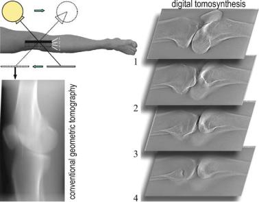
|
3 Milestones of Computed Tomography |
Fig. . . The first attempts to create radiographic slices of the human body were carried out using conventional or analog geometric tomography, also referred to as tomosynthesis if the acquired X-ray images are digitally post-processed. In this process, the X-ray tube and the detector are synchronously moved in opposite directions. For this reason, structures situated above and below the plane of the center of rotation are blurred (tomosynthesis images of a knee phantom: Courtesy of Siemens Medical Solutions (Härer et al. , ))
Table . . Historic milestones of analog tomography (see Webb )
Class |
Mechanical arrangement |
Motion |
Inventor |
Stratigraphy |
X-ray tube and film cassette |
Linear, |
Alessandro |
|
are perpendicular to a rigid |
circular |
Vallebona ( ) |
|
pivoting pendulum |
or spiral |
|
Planigraphy |
X-ray tube and film cassette |
Linear, |
André Edmond Marie |
|
move in parallel equidistant |
circular |
Bocage ( ), |
|
planes with reciprocal motions |
or spiral |
Ziedses des Plantes ( ), |
|
|
|
Ernst Pohl ( ) |
Tomography |
X-ray tube and film cassette |
Linear |
Gustav Grossmann ( ) |
|
are attached to a rigid pendu- |
|
|
|
lum, but the detector is always |
|
|
|
parallel to the tomographic |
|
|
|
plane |
|
|
|
|
|
|
enables a direct comparison between the analog image of the knee given by conventional geometric tomography (bottom left) and single slices acquired with a spacing of mm using tomosynthesis. The blurring angle, α, determines the extent to which

3.3 Rotation–Translation of a Pencil Beam (First Generation) |
|
the contribution from structures above and below the slice (S) are suppressed in the blurring. Besides the class of trajectory (see Table . ) of the X-ray tube (R) and detector (D), the blurring angle, α, determines the quality of the image at S. The larger the angle, α, the smaller the extrinsic slice artifacts, i.e., the amplitude of the signal from structures located exterior to the slice being reconstructed (Härer et al. ).
A related method, called “orthopan tomography,” is now widespread in dental radiology. In this method, a panoramic view of rows of teeth is produced on an imaging plane that is curved to follow the jaw. However, sophisticated trajectories allow a reconstruction of slices by geometric tomography as well.
Nowadays, the term “tomography”, despite competitive modalities such as MRI (magnetic resonance imaging) or PET (positron emission tomography), is still most commonly associated with computed tomography (CT) or, more precisely, with X-ray CT. CT is also referred to as CAT (computerized axial tomography) .
Computed tomography avoids the superimposition of blurred planes and produces such a large contrast that even soft tissue can be imaged well. The resulting leap in the quality of diagnostic imaging led to the enormous success of CT.
Historically, four distinct generations of CT have emerged. Their classification relates to both the way that X-ray tubes and detectors are constructed, and the way that they move around the patient. Figures . , . , . , and . illustrate the different generations schematically.
3.3
Rotation–Translation of a Pencil Beam (First Generation)
The first generation of CT involves an X-ray tube that emits a single needle-like X-ray beam, which is selected from the X-ray cone by means of an appropriate pinhole collimator. This geometry is referred to as “pencil beam”. A single detector is situated on the opposite side of the measuring field and the X-ray tube. The detector is moved synchronously along with the X-ray tube. This displacement is linear and is repeated for di erent projection angles, γ (cf. Fig. . ). Depending on the specific attenuation properties of the tissue, the intensity of the X-ray is attenuated on its path through the body.
The amount of X-ray attenuation is measured by the detector and subsequently digitally recorded. For each angle, γ, this step yields a simple one-dimensional radiograph. However, from this initial radiograph, it is still not possible to determine the spatial distribution of the tissue attenuation coe cients. It is clear that in order to determine the location of two consecutive objects on one projection line, the situation needs to be viewed sideways as well. This is the approach taken by CT. CT views an object from all sides, since the projection angle is varied from to .
In the early years terms like Computerized Transaxial Tomography (CTAT) or Digital Axial Tomography (DAT) were used (Bushong ).

|
3 Milestones of Computed Tomography |
|||||||
|
|
|
|
|
|
|
|
|
|
|
|
|
|
|
|
|
|
|
|
|
|
|
|
|
|
|
|
|
|
|
|
|
|
|
|
|
|
|
|
|
|
|
|
|
Fig. . . The first generation of CT is equipped with a pencil beam and a single detector. These are moved linearly, and the configuration is rotated through di erent projection angles, γ. Each point inside the field of view needs to be X-rayed from all “sides,” so the X-ray source and detector are rotated through . The X-ray pencil beam is extracted from the beam characteristic of the source, by using an appropriate pin-hole collimator
Fig. . . The first head scanner was built in the EMI Central Research Laboratories in London. Courtesy of General Electric Medical Systems
3.3 Rotation–Translation of a Pencil Beam (First Generation) |
|
The first CT scanner, built by the company EMI (Electric and Musical Industries Ltd.), was based on this principle. In Godfrey N. Hounsfield realized the scanner in the EMI Central Research Laboratories (Hounsfield ). For his invention, he jointly won the Nobel Prize for medicine together with Allen M. Cormack in. Figure . shows a picture of the EMI head scanner. The first experiments by
Fig. . . Hounsfield’s historic experiment, which he established in London at the EMI Central Research Laboratories in the s (top) and the first image produced (bottom). Courtesy of General Electric Medical Systems
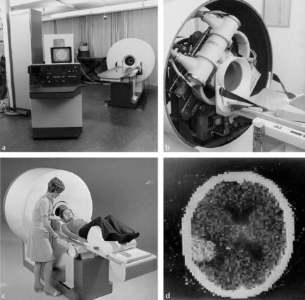
|
3 Milestones of Computed Tomography |
|
Hounsfield were performed in with a radioactive Americium source ( Am) |
|
being linearly displaced along with the detector. Hounsfield collected data in steps |
|
of , through the necessary for image reconstruction. The first reconstruc- |
|
tion of a two-dimensional slice took days – a clinically unacceptable processing |
|
time. However, for the first time, a two-dimensional slice image could be achieved |
|
that did not originate from averaging or blurring information, as in conventional |
|
geometric tomography mentioned in the section above. Figure . shows the his- |
|
torical layout of the experiment (top) as well as the first image it produced (bot- |
|
tom). |
Fig. . . One of the first commercially available, first-generation CT scanners was the Siemens Siretom in , shown here a closed and b with covers removed. With this scanner it was possible to produce c axial images of the head with d an image matrix of pixels. Courtesy of Siemens Medical Solutions

3.4 Rotation–Translation of a Narrow Fan Beam (Second Generation) |
|
The actual reconstruction of a two-dimensional slice is only possible if the projection values are digitized. The image section to be visualized is determined by the measurement principle, since the pencil beam virtually cuts the object at that slice. However, the calculation of the spatial distribution of the attenuation values at that very slice is mathematically complex and will be described in Chaps. – . Due to the complexity of the mathematical methods of Johann Radon’s reconstruction technique, published in , it remained only theory for half a century. A practical solution to the reconstruction problem was not possible until the development of computer technology . It is from this that CT gets its name.
The first commercial scanners from EMI had a narrow focused X-ray beam and a single sodium iodide (NaI) scintillation detector. This pencil-beam principle, which is not practiced any more, is of fundamental importance as it is here that the mathematical methods of reconstruction can be understood most easily. Indeed, the mathematical methods of more modern geometries can be obtained from pencil-beam geometry using suitable coordinate transformations. Figure . shows one of the first tomographs of the first generation produced by Siemens in . The subsequent rapid development of CT has been, and still is, driven by three essential goals: Reduction of acquisition time, reduction of X-ray exposure, and, last but not least, reduction of cost. Throughout the course of optimizing these factors there are several historical stages, which are briefly described in the following sections.
3.4
Rotation–Translation of a Narrow Fan Beam (Second Generation)
The computed tomograph of the second generation has an X-ray source with a narrow fan beam and a short detector array consisting of approximately elements (cf. Fig. . ). However, since the aperture angle of the fan beam is small, the X-ray tube and detector array still need to be translated linearly before the projection angle is adjusted for another projection. In the earliest of the second-generation scanners, the angle of the fan beam was about .
Despite the need for linear displacement, the acquisition time was reduced to a few minutes per slice, as the detector array could measure several intensities simultaneously. However, the measuring field was still small. For this reason, and due to their long acquisition times, the firstand second-generation scanners were mainly restricted to use in imaging the cranium. Figure . c gives an idea of the scale of the measuring field. The cranium can be fixed in the scanner and shows no large intrinsic movement during acquisition time (relative to the spatial resolution that could be achieved at the time).
In Sect. . , it is shown that this is not entirely historically correct. In , Edholm ( ) proposed an analog, optical procedure for tomographic image reconstruction.

|
3 Milestones of Computed Tomography |
Fig. . . The CT scanners of the second generation have one X-ray source with fan-beam geometry, as well as a short detector array. The X-ray fan is created from a conical X-ray source by means of a slit-shaped collimator. The fan angle is about and the detector is made up of elements. In this case, the detector and tube also need to be moved linearly before the projection angle is adjusted, as the entire field of view is not X-rayed by the fan
This is certainly not the case when imaging the area of the thorax or the abdomen, as the intrinsic movements of the heart and lung, as well as the movement of the diaphragm and soft organs of the abdomen, produce artifacts in the reconstructed images. The mathematical methods of reconstruction demand that all points of one slice are X-rayed from all angles from through . One object moving out of the imaging plane during rotation of the X-ray tube, due to patient movement, will inevitably result in errors in image reconstruction. Such image errors, referred to as motion artifacts, are described in detail in Chap. .
3.5
Rotation of a Wide Aperture Fan Beam (Third Generation)
The main goal of developments in the s was to reduce acquisition time down to less than s. This was intended to give enough time to acquire an image of the abdomen with minimal error, while the patients held their breath. A major step toward achieving this goal was an extension of the second generation’s fan-beam
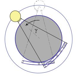
3.5 Rotation of a Wide Aperture Fan Beam (Third Generation) |
|
concept, i.e., the introduction of a substantially larger angle of the X-ray fan and a correspondingly longer detector array. Figure . gives a schematic illustration of this principle of third-generation scanners.
Nowadays, the angle of an X-ray fan beam is typically between and and the detector array is usually constructed as an arc with between and ,
elements. In this way it is now possible to simultaneously X-ray the entire measuring field, which is currently wide enough to cover the torso, for each projection angle, γ. As a result, the third generation of CT systems can completely abandon linear displacement of the X-ray tube. The acquisition time for third-generation systems is reduced considerably, since a continuous rotation can take place without interruption for linear displacement. The majority of CT scanners currently in use are fan-beam systems of the third generation. Figure . shows an experimental set-up of a third-generation scanner with a mechanical magnification unit in the Philips research labs and Fig. . shows a typical Siemens CT scanner of .
Fig. . . The third generation of CT scanners has a substantially larger angle of the X-ray fan and a longer detector array, such that the entire measuring field can be X-rayed simultaneously for one single projection angle, γ. Hence, the need for linear displacement of the source-detector system is removed. The third generation represents an extension of the principle behind the second generation. The fan angle is usually around to and the detector array is made of up to , detector elements. As a consequence of the larger aperture, the X-ray is exploited to a greater extent. Also, the scanner can rotate continuously without stopping for linear displacement. This results in a major reduction of acquisition time

|
3 Milestones of Computed Tomography |
Fig. . . a Principle of geometric enlargement in . Two possible positions of the tube/detector construction as to optimize the scanner for both head and body scan, while having a limited detector size. b Detector module of channels. c Lab model including geometric enlargement construction. Courtesy of Leon de Vries, Philips Medical Systems
Typical image errors of third-generation scanners are called “ring artifacts.” A single defective, or even insu ciently calibrated, detector in the array results in characteristic ring-shaped errors in the reconstructed tomogram. These kinds of
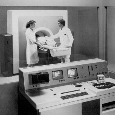
3.6 Rotation–Fix with Closed Detector Ring (Fourth Generation) |
|
Fig. . . An example of a whole body scanner from : The Siemens Somatom family DR. This third generation of computed tomography scanners has a measuring field of approximately cm in diameter. With solid state detectors, acquisition times of about s were possible for a rotation (courtesy of Siemens Medical Solutions)
artifacts are discussed in detail in Sect. . . . While they are seen in images from third-generation scanners, they cannot appear in images from fourth-generation tomographs.
3.6
Rotation–Fix with Closed Detector Ring (Fourth Generation)
The fourth generation of CT scanners does not di er from the third-generation tomographs with respect to the X-ray tube. The fan-beam source also rotates continuously around the measuring field without any linear displacement. The di erence is in the closed, stationary detector ring with up to , single elements. The X-ray tube either rotates outside (Fig. . , left) or inside (Fig. . , right) the detector ring.

3 Milestones of Computed Tomography
Fig. . . Computed tomography scanners of the fourth generation do not di er from those of the third generation with respect to the X-ray source. As with the third generation, the X-ray source rotates continuously without any linear displacement. However, the fourth generation has a stationary detector ring. Within the fourth generation systems there are two distinct types: The path of the X-ray source is either outside (left) or inside (right) the detector ring. The number of detectors is around , . The angle of the fan beam depends on the measuring field
Fig. . . The fourth generation of CT scanners uses an “inverse fan,” whose center is situated at a single detector. Unlike the third-generation scanners, it is in principle possible to measure an arbitrarily dense inverse fan, as long as a single detector element can be read at a high enough frequency while the X-ray source moves continuously
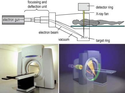
3.7 Electron Beam Computerized Tomography |
|
If the X-ray tube is outside the detector ring, it is necessary to prevent the X-rays from radiating through the detectors from behind. Therefore, the detector ring is dynamically tilted away from the path of the tube. In this way, the line of sight between the tube and the appropriate section of the detector ring only passes through the patient (and patient table) and not through the electronics behind the detectors.
The fourth-generation tomographs establish “inverse fans,” which are centered on detectors rather than on the X-ray focus. Figure . shows an inverse fan schematically. An inverse fan is also referred to as a “detector fan.”
An inverse fan can be very dense, limited only by the sampling rate at which individual detectors can be read out. As a result, unlike third-generation tomographs, this scanner is not limited to the spatial resolution of a single fan beam.
3.7
Electron Beam Computerized Tomography
If there is a need for even shorter acquisition times, the concept of moving sampling systems must be left behind entirely. One approach to achieving this is using electron beam computerized tomography (EBCT). This type of CT was developed for cardiac imaging.
Fig. . . Realization of an electron beam computerized tomography (EBCT) scanner by Imatron, for fast cardiac imaging. Courtesy of General Electric Medical Systems

|
3 Milestones of Computed Tomography |
|
|
In EBCT, there is no longer a localized X-ray tube rotating around the patient |
|
|
as in conventional CT technology. Instead the patient is situated, in a manner of |
|
|
speaking, inside the X-ray tube. An electron beam is focused onto wolfram target |
|
|
rings, which are arranged in a half circle around the patient, and generates the de- |
|
|
sired X-ray fan beam upon impact with the wolfram target. The X-ray irradiation |
|
|
is measured with a stationary detector ring. |
|
|
Such systems have mainly been sold to cardiologists by the company Imatron. |
|
|
T he electron beam technique is able to acquire an image slice in ms. Figure . |
|
|
shows a diagram of an EBCT system as well as an illustration of a modern Imatron |
|
|
system. Further technical details can be found, for example, in Weisser ( ). |
|
3.8
Rotation in Spiral Path
Another development, which was a great leap forward in capability from that of the third generation, led to what is identified by Bushberg et al. ( ) as the sixth generation of tomography scanners. This refers to the introduction of slip-ring technology, which enables spiral or helical sampling respectively.
As the X-ray tube must be continuously supplied with energy, the rate of circular movement was previously limited by the attachment of an electric cable, which was mounted on a spool. In this process the cable was unwound in one direction and carefully wound up in the other. This represented a huge obstacle to the reduction of acquisition time. The X-ray sampling unit had to stop and start again after a certain angle of rotation. Although data could be collected throughout both clockwise and counter-clockwise rotations, limits were placed on high velocities due to the increasing torsional moment. This problem was solved by the introduction of slip-ring technology. In this technology, the energy is provided via sliding contacts, situated between the outside of the sampling unit, in what is called the gantry, and the rotating sampling unit. This enables the sampling unit carrying the X-ray source and, in the case of third-generation scanners, the detector array, to rotate continuously. As a result of slip-ring technology, rotation frequencies of two rotations per second, “sub-second scanners”, are nowadays commonplace.
Figure . shows di erent technologies for the transfer of energy. On the left, slip-ring technology, as discussed above, can be seen on a Siemens Somatom AR.T CT scanner. However, there are also smaller, more compact devices, in which the sampling unit is independent from an external energy supply during rotation, by means of accumulators. An example is given on the right of Fig. . , which shows a mobile Philips Tomoscan M CT scanner with the covers removed.
The slip-ring innovation enabled a new acquisition technique. Along with a continuous motion of the patient table through the sampling unit, it became possible to measure data in the shape of a spiral . The spiral-CT technique was demonstrated
Strictly speaking, the X-ray tube trajectory is a helix.
3.9 Rotation in Cone-Beam Geometry |
|
Fig. . . Di erent methods of energy transfer to the continuously rotating sampling unit. In the Siemens Somatom AR.T (left), slip-ring technology is used. In the compact mobile CT scanner of the Philips Tomoscan M (right) an accumulator array is used
Fig. . . Willi Kalender in the mid- s at the Laboratories of Siemens (by courtesy of W. Kalender)
successfully on a prototype by Kalender in (Kalender et al. ). Figure . shows Willi Kalender at the laboratories of Siemens Medical Solutions in the mid-
s.
3.9
Rotation in Cone-Beam Geometry
As already mentioned, there has so far not been a common definition of the generations of development of CT. In Bushberg et al. ( ), scanners equipped with

|
3 Milestones of Computed Tomography |
|
|
|
|||
|
a cone-shaped X-ray beam and a plane detector are referred to as the seventh gen- |
||||||
|
eration. |
|
|
|
|
|
|
|
However, even within the cone-beam scanner itself, one needs to distinguish |
||||||
|
between systems that use only a small cone opening, as in the case of a multi- |
||||||
|
slice (multi-line) detector system or indeed a symmetric X-ray cone. In particular, |
||||||
|
the necessary reconstruction methods di er extensively between these systems, as |
||||||
|
To |
|
|
Chap. . |
|
|
|
|
demonstrated in |
|
|
|
|
||
|
|
understand the motivation behind the development of cone-beam CT sys- |
|||||
|
tems, recall that the step from the pencil-beam to the fan-beam concept came along |
||||||
|
with the advantages that the X-ray source was exploited more e ectively, and that |
||||||
|
there was a reduction in acquisition time. In |
|
Sect. . . it has been discussed that |
||||
|
the e ciency of the energy transformation |
throughout the generation of X-ray ra- |
|||||
|
|
|
|
||||
diation is just about %.
As the heat produced inside the X-ray tube essentially defines the physical capacitance, and therefore limits the measuring time, the next straightforward step in the development of CT scanners involved the use of a cone-shaped X-ray beam, which is already produced in the X-ray tube. Both the pencil-beam and the fanbeam geometry are created by means of appropriate pin-hole or slit collimators, which re-shape the original X-ray source intensity profile, reducing e ciency.
Technologically, there are three important problems that had to be solved before the successful application of cone-beam geometry to CT imaging.
Fig. . . Prototype of a cone-beam CT scanner, equipped with a flat detector. Courtesy of Siemens Medical Solutions

3.10 Micro-CT |
|
First of all, a flat-panel detector, which did not exist at the time, had to be introduced to replace the line or multi-line detector arrays. Second, the huge amount of raw data that quickly emerge on sub-second scanners in particular had to be transferred from the rotating sampling unit to the image reconstruction computer. The required bandwidth for the data transfer poses a challenge even today. Third, there is the problem of reconstruction, whose mathematics is slightly more sophisticated compared with the two-dimensional methods. This will be discussed in detail inChap. . Figure . shows a prototype of a cone-beam CT scanner at the Siemens laboratories.
3.10 Micro-CT
Recently, micro-CTs, which essentially comprise a miniaturized design of the conebeam CTs mentioned in the previous section, and which are typically used for nondestructive, three-dimensional microscopy, have become commercially available. The X-rayed measuring field, usually as small as cm in volume, is so small that medical applications might seem to be ruled out. Indeed, these scanners are more commonly used for material testing and analysis, but medical applications are on their way to taking center stage. An example in human medicine is the analysis of trabecular structures in bones. Micro-CTs are also ideal scanners for radiological examinations of small animals (De Clerck et al. ).
Figure . shows a commercial micro-CT system, manufactured by the Belgian company SkyScan. It is produced as a desktop device and has a measurement chamber that is entirely shielded against scattered X-ray beams by lead walls, so that no further means of protection are necessary. The object to be examined is placed on a rotating specimen disk, which is controlled by a step motor.
Figure . a shows the preparation of an examination of a Neanderthal man’s tooth. This specimen is about , years old. The curator of the Department of Preservation of Archeological Monuments in Koblenz is currently interested in the structure of the tooth’s interior. Figure . b shows a cone-beam X-ray of the tooth. As well as the nerve channel, the fissure lines are imaged very well.
The two most crucial components of micro-CTs are the X-ray tube and the twodimensional detector array. In particular, it is the size of the focus and the size of the detector elements that, apart from the mechanical accuracy of the rotary motion, determine spatial resolution. In Fig. . it has already been illustrated how the size of the focus a ects the representation of detail. It follows that the micro-CT system
needs a micro-focus tube. In |
|
Sect. . it will be shown that it is the modulation |
|||||||||||||
transfer function, |
|
|
|
|
( |
|
) |
9 9 |
( |
|
|
|
) |
|
|
( )= |
|
|
( ) |
( )=9 |
|
F |
|
D |
|
|
|||||
MTFimaging system q MTFX-ray source |
q MTFdetector q |
sin |
|
πbF q |
|
|
sin |
πbD q |
|
|
|||||
|
|
|
|
|
πb q |
|
|
πb |
|
q |
|
|
|||

|
3 Milestones of Computed Tomography |
Fig. . . a Micro-CT desk device of SkyScan Inc. at the Institute of Medical Engineering, University of Lübeck, Germany. The object to be examined is placed on a rotating specimen holder inside the measurement chamber. The measurement field is about cm in volume. b A simple X-ray image of a tooth from an archeological dig illustrates an impressive variety of structures. As well as the nerve channel, fine fissure lines that have been formed inside this Neanderthal man’s tooth over the millennia are recognizable. The small arrow indicates the location of a reconstructed slice, which will be examined in more detail. The planar ,, pixel charge-coupled device (CCD) array is cooled down and has a detector size of bD < μm
that quantifies the resolution of objects with a spatial frequency q (given in line pairs per millimeter). In the case of micro-CTs, an X-ray focus size of bF < μm is desirable. Using such a small target area for the electrons, the anode current cannot be very large. The current is typically less than μA. Since the current controls the intensity of the X-ray spectrum, there are certain constraints with respect to the materials being examined. A -bit X-ray charge-coupled device (CCD) chip with a pixel matrix of , , is used as a detector, which is connected to the scintillation crystal by fiber optics. The size of the picture elements has an order of magnitude of around bD < μm. SkyScan specifies a resolution of about μm (Sassov , a, b). As micro-CTs are cone-beam X-ray systems, threedimensional reconstruction methods are required to calculate the images (Wang et al. ).
Figure . shows the di erence in spatial resolution between a micro-CT and a clinical CT system, using the example of the tooth from a Neanderthal man. In a reconstructed slice, fine fissures are identifiable in the image from the micro-CT (Fig. . a). The reconstruction using a clinical CT (Fig. . b) is not able to resolve these details. The location of the section shown in Fig. . a,b is marked with an arrow in Fig. . b. When comparing the three-dimensional reconstructions and
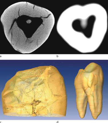
3.10 Micro-CT |
|
Fig. . . Comparative inspection of image resolutions, using the example of the tooth from an archeological dig. An approximately , -year-old Neanderthal man’s tooth was examined using a, c micro-CT and b, d ordinary clinical CT. The position of the reconstructed section is marked in Fig. . b. The di erence is immediately obvious. The fine fissures that have formed inside the tooth over the millennia cannot be imaged using clinical CT. c In the three-dimensional reconstruction of the micro-CT image the fissures can be identified as fissure planes. For comparison, the entire tooth imaged by the ordinary CT scanner has been reconstructed in d. Given the dimensions of the tooth, even this reconstruction is impressive, but it does not reveal the micro-structures evident in the micro-CT image
visualizations in Fig. . c,d, there is a distinct di erence as well. Fissure planes passing through the entire tooth are only visible on the micro-CT image.

3 Milestones of Computed Tomography
3.11
PET-CT Combined Scanners
With the exception of contrast-enhanced angiography and perfusion techniques, CT, on its own, is only able to provide morphological information, i.e., information on the shape of objects. On the other hand, positron emission tomography (PET) provides information on the metabolism, i.e., the biomedical function of an anatomical region. As already described in Chap. , CT is based on the attenuation of X-ray radiation. Di erent organs, having di erent absorption properties, are therefore only imaged according to their shape, and the patient is considered to be passive during imaging.
In PET, the patient is injected with a radioactively marked tracer, which is metabolized inside the body. One very important tracer is F-FDG ( −(Fluorine- - Fluoro- -Deoxy-D-Glucose), which can be used to trace glucose metabolism. This is especially important for oncology studies, since, due to their faster metabolism, theF-FDG uptake of tumors exceeds the uptake of non-malignant tissue. Compared with ordinary glucose, F-FDG di ers in the presence of the tracer atom. As such, it behaves like glucose only at the beginning of the metabolic chain. T hereaf ter, the molecule is detected, but not catabolized any further, leading to an accumulation of the tracer inside the tumor.
F-FDG is a positron emitter , so wherever the tracer accumulates, the process of positron annihilation is intensified. This process was shown as a daughter process of pair production in Fig. . , and is described by ( . ). In the case of F-FDG, however, a proton, p, decays into a neutron, n, a neutrino, ν, and a positron, e+, as a parent process
p n + e+ + ν . |
( . ) |
Upon collision with an electron close to where this decay occurs, the positron entirely de-materializes, becoming two gamma ray photons that fly away in opposite directions. The gamma ray photons are then measured by two detectors, located opposite each other, in what is called a coincidence measurement. By means of filtered backprojection, the location of the de-materialization can be reconstructed, and tumors are represented as hot spots inside the image. The mathematical fundamentals of the image reconstruction of PET techniques will be described later. For further details of the technique, and of applications of PET, the reader is referred, for example, to Ruhlmann et al. ( ).
An interesting approach to imaging diagnostics is the combination of both morphological and functional imaging methods. The goal of displaying function along with morphology in a single image has been realized for some time using methods of image registration . Registration is an image processing step that must over-
Positrons, e+, are the antiparticles of electrons, e−.
Registration is an image processing step, aligning the coordinate systems of two modalities. A detailed illustration of these techniques can be found, e.g., in Hajnal et al. ( ).
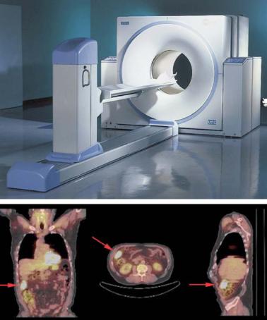
3.11 PET-CT Combined Scanners |
|
come problems caused by the di erent positioning of the patient in two di erent scanners, and changes resulting from the time that passes between the two acquisitions.
In the case of combined techniques, the patient is successively scanned using the di erent imaging modalities. Using a combined PET-CT scanner, such as, for instance, the biograph from Siemens (Fig. . , top), the images are acquired almost simultaneously, with the patient e ectively in the same position, so that the location of a tumor relative to the surrounding anatomy can be displayed immediately. The bottom of Fig. . shows an intestinal tumor being imaged as a hot spot.
Fig. . . The biograph scanner from Siemens is an integrated PET-CT concept that can image metabolic and anatomic information at the same time. Courtesy of Siemens Medical Solutions

3 Milestones of Computed Tomography
3.12
Optical Reconstruction Techniques
The term “computed tomography” is historically connected to the development of computers, which have been successfully applied in the field of image reconstruction since the s. It was mentioned in Sect. . , that a practically applicable solution to the problem of image reconstruction was not possible before the introduction of computer technology. In fact, there is also the possibility of achieving reconstruction in an optico-photographic fashion. In Edholm introduced a tricky optical configuration, which is illustrated in Fig. . .
In order to acquire an image, an X-ray fan is produced using slit collimation, which radiates through the object and whose projection profile is recorded on a film as a single line. The film is moved linearly and synchronously with the rotation of the object being examined.
The resulting pattern is referred to as a sinogram, and can be used for reconstruction. The first step in the reconstruction chain is the one-dimensional illumination of the sinogram, which is imaged by a cylinder lens onto a second film. The cylinder lens spreads the profile spatially. By displacing the sinogram film and
Fig. . . Principle of the optical reconstruction method for analog CT based on the ideas of Edholm ( )
3.12 Optical Reconstruction Techniques |
|
simultaneously rotating the cylindrical lens, a simple backprojection is achieved since all projection profiles are superimposed. In a final step the resulting backprojection is high-pass filtered using Fourier optics to produce the image reconstruction. Nowadays, computer technology is so advanced, that results are superior to those of optical reconstruction. Therefore, optical techniques are no longer pursued.